Signal visualisation
Learning outcomes
Using
deepToolsto visualise ChIP / ATAC signal in relation to annotated TSSUsing
pyGenomeTracksto plot genome browser tracks
Before we start
Analysis of ATAC/ ChIP-seq data wouldn’t be complete without visualising the signal in many ways at various stages of the analysis.
Signal can be visualised and summarised in relation to annotated features, such as in deepTools part of this tutorial, and this may serve as a diagnostic tool (i.e. we expect to see higher density of signal in transcription start site regions), for data exploration (i.e. we can detect features with various signal distribution patterns) or for plotting final figures.
We can also use tools to produce visually attractive plots of genomic tracks, such as ones we have inspected using Integrative Genome Browser during the tutorials. We show you how to start with these type of visualisations in section on pyGenomeTracks.
In both cases the options for plot customisation are many, and we encourage you to explore the parameters.
Signal visualisation with deepTools
We can visualise signal in relation to annotated features.
One such kind of features relevant for TFs are transcription start sites (TSS). In this exercise we use ChIP-seq data from ChIPseq lab. The data we are going to plot is from one replicate of ChIP-seq experiment investigating binding of REST transcriptional represssor in HeLa cells. and annotations for chromosomes 1 and 2. To do so we will:
produce coverage track in
bedgraphformat;convert
bedgraphtobigWigusingUCSC utilities;calculate scores per genome regions using the
bigWigfile;plot a heatmap of scores associated with genomic regions
Setting up
We first link necessary files. Assuming we are in the home directory:
mkdir vis
cd vis

mkdir deepTools
cd deepTools

ln -s /proj/epi2025/chipseq_processing/hg19/chrom.sizes.hg19
ln -s /proj/epi2025/chipseq_processing/hg19/refGene_hg19_TSS_chr12_sorted_corr.bed
ln -s /proj/epi2025/chipseq_processing/data/bam/hela/ENCFF000PED.chr12.rmdup.sort.bam
ln -s /proj/epi2025/chipseq_processing/data/bam/hela/ENCFF000PED.chr12.rmdup.sort.bam.bai
Normalised coverage tracks
Let’s start from generating a normalised coverage track in a format called bedgraph from bam file. The bam file contains data subset to chr1 and chr2, hence we use effectiveGenomeSize 492449994 (length of chr1 and chr2). The data is SE, so we extend the reads to average fragment length
..(which we know from the Cross correlation)
(which we know from the Cross correlation)
using parameter --extendReads 110. Last but not least, we scale the track to average 1x coverage using option --normalizeUsing RPGC.
#if required
module load bioinfo-tools

module load deepTools/3.3.2

bamCoverage --bam ENCFF000PED.chr12.rmdup.sort.bam \
 --outFileName ENCFF000PED.chr12.cov.norm1x.bedgraph \
 --normalizeUsing RPGC --effectiveGenomeSize 492449994 --extendReads 110 \
 --binSize 50 --outFileFormat bedgraph
This track can be used for various visualisations and comparisons.
We can convert it to another format bigWig:
module load ucsc-utilities/v398

bedGraphToBigWig ENCFF000PED.chr12.cov.norm1x.bedgraph chrom.sizes.hg19 hela_1.bw

module unload ucsc-utilities
Hint
If these above steps did not work, you can link the precomputed coverage tracks:
ln -s /proj/epi2025/chipseq_processing/results/coverage/hela_1.bw
ln -s /proj/epi2025/chipseq_processing/results/coverage/ENCFF000PET.cov.norm1x.bedgraph
Plotting signal in relation to TSS
We begin by summarising coverage in bins in relation to a set of reference points, TSS in our case.
We can compute the matrix of scores for visualisation using computeMatrix. This tool calculates scores per genome regions and prepares an intermediate file that can be used with plotHeatmap and plotProfiles.
Typically, the genome regions are genes (or TSS as in this case), but any other regions defined in a BED file can be used. computeMatrix accepts multiple score files (bigWig format) and multiple regions files (BED format). This tool can also be used to filter and sort regions according to their score.
module load deepTools/3.3.2

computeMatrix reference-point -S hela_1.bw \
-R refGene_hg19_TSS_chr12_sorted_corr.bed -b 5000 -a 5000 \
--outFileName matrix.tss.dat --outFileNameMatrix matrix.tss.txt \
--referencePoint=TSS -p 10
We can now create a heatmap for scores associated with genomic regions, i.e. plot the binding profile around TSS
plotHeatmap --matrixFile matrix.tss.dat \
--outFileName tss.hela_1.pdf \
--sortRegions descend --sortUsing mean
tss.hela_rep1.pdf
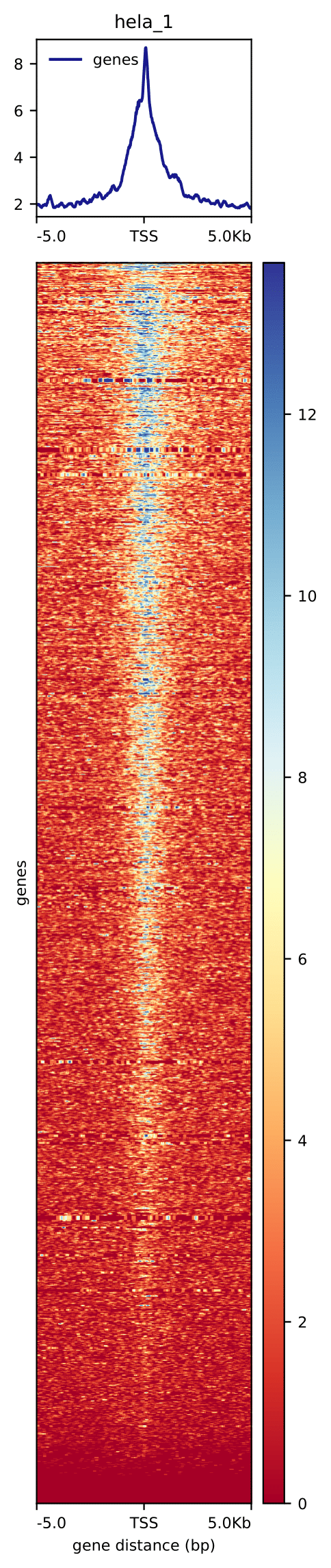
Have a look at tss.hela_rep1.pdf. Can this plot be improved?
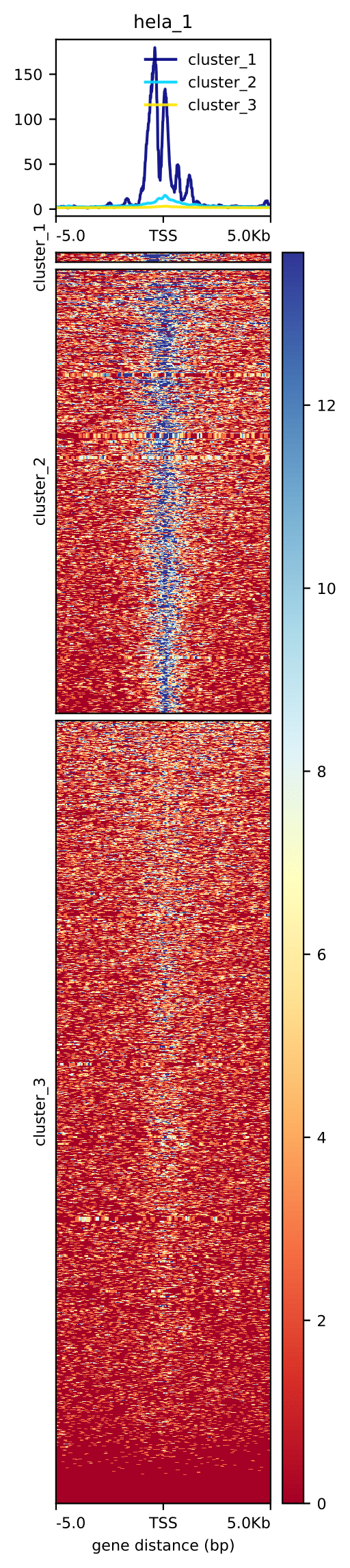
This is a very basic plot. We can add on to it, for example we can cluster genes based on the signal profile around TSS. For more possibilities please check plotHetmap.
plotHeatmap --matrixFile matrix.tss.dat \
--outFileName tss.hela_rep1_k3.pdf \
--sortRegions descend --sortUsing mean \
--kmeans 3
tss.hela_rep1_k3.pdf
You can also use the same tools to plot signal along a scaled gene body using computeMatrix scale-regions. More examples are given on deepTools homepage.
Plotting Tracks using pyGenomeTracks
pyGenomeTracks can be used to plot browser tracks in multiple formats. In this tutorial we will plot ATAC-seq data from ATACseq lab along with detected peaks and gene models.
The process has two steps, first we define the formats in file track.ini and next we plot the desired regions. Although there is a learning curve to using pyGenomeTracks, and it often requires few tries to get the settings right, this is a convenint and reproducible manner to produce identically formatted plots of multiple regions.
Let’s link the necessary files and produce coverage tracks (assuming we are in vis):
mkdir pyGT
cd pyGT

ln -s /sw/courses/epigenomics/2022/vis/pyGT/ENCFF398QLV.chr14.norm1x.bedgraph
ln -s /sw/courses/epigenomics/2022/vis/pyGT/ENCFF045OAB.chr14.norm1x.bedgraph

ln -s /sw/courses/epigenomics/2022/vis/pyGT/nk_genrich.bed
ln -s /sw/courses/epigenomics/2022/vis/pyGT/nk_stim_genrich.bed
ln -s /sw/courses/epigenomics/2022/vis/pyGT/nk_macs_broad.bed
ln -s /sw/courses/epigenomics/2022/vis/pyGT/nk_stim_macs_broad.bed
ln -s /sw/courses/epigenomics/2022/vis/pyGT/ENCFF045OAB.macs.broad_peaks.broadPeak
ln -s /sw/courses/epigenomics/2022/vis/pyGT/ENCFF045OAB.genrich.narrowPeak
ln -s /sw/courses/epigenomics/2022/vis/pyGT/ENCFF398QLV.macs.broad_peaks.broadPeak
ln -s /sw/courses/epigenomics/2022/vis/pyGT/ENCFF398QLV.genrich.narrowPeak

ln -s /sw/courses/epigenomics/2022/vis/pyGT/hg38.refGene.gtf

cp /sw/courses/epigenomics/2022/vis/pyGT/tracks1.ini .
cp /sw/courses/epigenomics/2022/vis/pyGT/tracks2.ini .
Hint
bedgraph tracks were created with smaller bins, no smoothing:
module load bioinfo-tools
module load deepTools/3.3.2

bamCoverage --bam ENCFF045OAB.chr14.proc.bam \
 --outFileName ENCFF045OAB.chr14.norm1x.bedgraph \
 --normalizeUsing RPGC --effectiveGenomeSize 107043718 \
 --binSize 10 --outFileFormat bedgraph

bamCoverage --bam ENCFF398QLV.chr14.proc.bam \
 --outFileName ENCFF398QLV.chr14.norm1x.bedgraph \
 --normalizeUsing RPGC --effectiveGenomeSize 107043718 \
 --binSize 10 --outFileFormat bedgraph
You can create tracks using other settings, combining bin size and smoothing settings. You will need:
ln -s /proj/epi2023/vis/pyGT/ENCFF045OAB.chr14.proc.bam
ln -s /proj/epi2023/vis/pyGT/ENCFF045OAB.chr14.proc.bam.bai
ln -s /proj/epi2023/vis/pyGT/ENCFF398QLV.chr14.proc.bam
ln -s /proj/epi2023/vis/pyGT/ENCFF398QLV.chr14.proc.bam.bai
We can now create the track.ini file. You can check possible options in compatible tracks
We will visualise the following:
data as bedgraph
peaks as bed (narrowPeak and broadPeak)
gene models as gtf
We need to know the paths to files, let’s check the current directory:
pwd
In my case it was /proj/epi2022/nobackup/agata/tests/vis/pyGT, yours will be different, so substitute acccordingly.
Let’s build a simple ini file:
[x-axis]
where = top

[spacer]
height = 0.3

[bedgraph]
file = /proj/epi2022/nobackup/agata/tests/vis/pyGT/ENCFF398QLV.chr14.norm1x.bedgraph
# height of the track in cm (optional value)
height = 4
title = ATAC-seq NK
color = mediumturquoise
min_value = 0

[spacer]
height = 0.3

[bedgraph]
file = /proj/epi2022/nobackup/agata/tests/vis/pyGT/ENCFF045OAB.chr14.norm1x.bedgraph
# height of the track in cm (optional value)
height = 4
title = ATAC-seq stimulated NK
color = forestgreen
min_value = 0

[spacer]
height = 0.5

[bed]
file = /proj/epi2022/nobackup/agata/tests/vis/pyGT/nk_genrich.bed
# height of the track in cm (optional value)
height = 4
title = consensus Genrich peaks in NK
color = lightpink

[spacer]
height = 0.3

[bed]
file = /proj/epi2022/nobackup/agata/tests/vis/pyGT/nk_stim_genrich.bed
# height of the track in cm (optional value)
height = 4
title = consensus Genrich peaks in stimulated NK
color = crimson

[spacer]
height = 0.5

[genes]
file = /proj/epi2022/nobackup/agata/tests/vis/pyGT/hg38.refGene.gtf
file_type = gtf
title = gene models
style = flybase
arrow_interval = 3
display = stacked
fontsize = 10
gene_rows = 10
height = 7
all_labels_inside = true
merge_transcripts = true
Hint
It is generally not advised to edit files used on Linux systems in word processing editors such as MsWord and similar (due to meta characters added by them for formatting purposes - they may not be visible, but they are present in text copied directly from such editors. For generating the *ini files in this example, and general script writing, it is recommended to use text editors developed for programming. Not only they do not add any invisible characters to the text, but often include convenient utilities such as syntax highlighting for a wide choice of programming languages.
One example of such editor is Sublime.
You can copy the contents of tracks.ini to the editor, modify the paths and paste back to rackham:
#create a file and open a simple editor
nano tracks.ini

# now copy the file contents

#to close and save the file
Ctrl-X
#to save under given name press Y, then "enter"
This file is available as tracks1.ini.
Hint: You can keep only the file names (not the full paths), if running the plotting from the same directory where the files are located.
pyGenomeTracks is installed via a conda environment, so we activate it first
#unloading module python may be necessary
module unload python
module load conda/latest
conda activate /sw/courses/epigenomics/software/conda/pygenometracks3_7
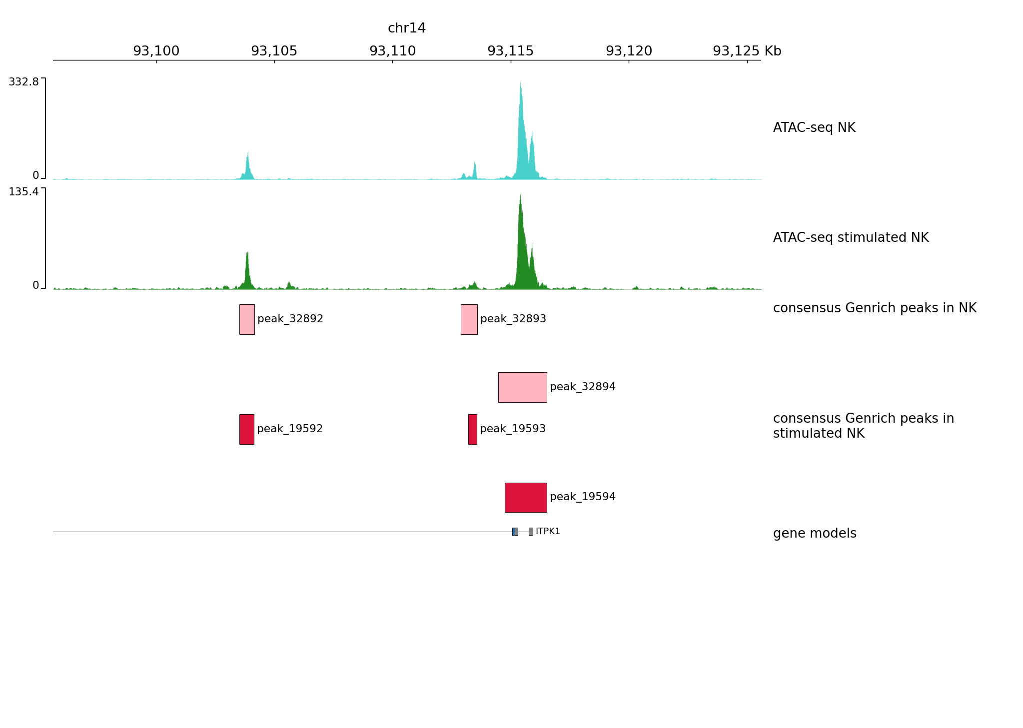
Let’s plot one of the regions we have viewed in the ATAC-seq peak detection part chr14:93,095,621-93,125,599
pyGenomeTracks --tracks tracks1.ini --region chr14:93095621-93125599 --trackLabelFraction 0.2 --dpi 130 -o plot1.png
plot1.png
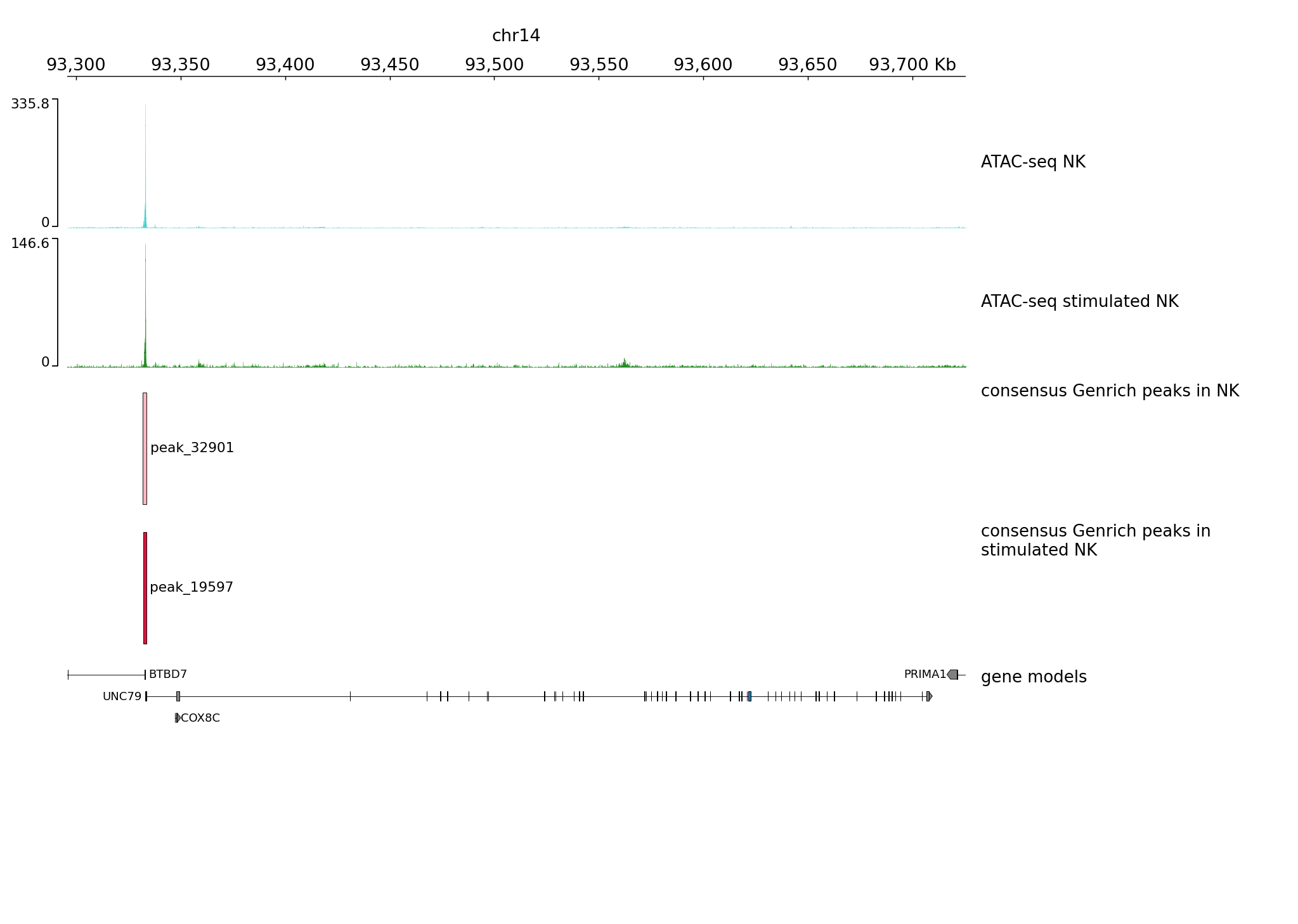
We can plot wider region using the same settings
pyGenomeTracks --tracks tracks1.ini --region chr14:93295621-93725599 --trackLabelFraction 0.2 --dpi 130 -o plot2.png
plot2.png
Let’s tweak some settings in the ini file.
We can add
max_valueto bedgraph tracks to use the same scale for both samples;We can change the style of gene models display to
style = UCSC
Modified file:
[x-axis]
where = top

[spacer]
height = 0.3

[bedgraph]
file = /proj/epi2022/nobackup/agata/tests/vis/pyGT/ENCFF398QLV.chr14.norm1x.bedgraph
# height of the track in cm (optional value)
height = 4
title = ATAC-seq NK
color = mediumturquoise
min_value = 0
max_value = 600

[spacer]
height = 0.3

[bedgraph]
file = /proj/epi2022/nobackup/agata/tests/vis/pyGT/ENCFF045OAB.chr14.norm1x.bedgraph
# height of the track in cm (optional value)
height = 4
title = ATAC-seq stimulated NK
color = forestgreen
min_value = 0
max_value = 600

[spacer]
height = 0.5

[bed]
file = /proj/epi2022/nobackup/agata/tests/vis/pyGT/nk_genrich.bed
# height of the track in cm (optional value)
height = 1
title = consensus Genrich peaks in NK
color = lightpink

[spacer]
height = 0.3

[bed]
file = /proj/epi2022/nobackup/agata/tests/vis/pyGT/nk_stim_genrich.bed
# height of the track in cm (optional value)
height = 1
title = consensus Genrich peaks in stimulated NK
color = crimson

[spacer]
height = 0.5

[genes]
file = /proj/epi2022/nobackup/agata/tests/vis/pyGT/hg38.refGene.gtf
file_type = gtf
title = gene models
style = UCSC
arrow_interval = 3
display = stacked
fontsize = 10
gene_rows = 10
height = 7
all_labels_inside = true
merge_transcripts = true
This file is available as tracks2.ini.
Hint
To modify a file we can use a simple text editor present on most unix / linux distributions nano.
Type nano tracks2.ini and you can edit the file. To save press Ctrl-X, confirm y, change file name if you like.
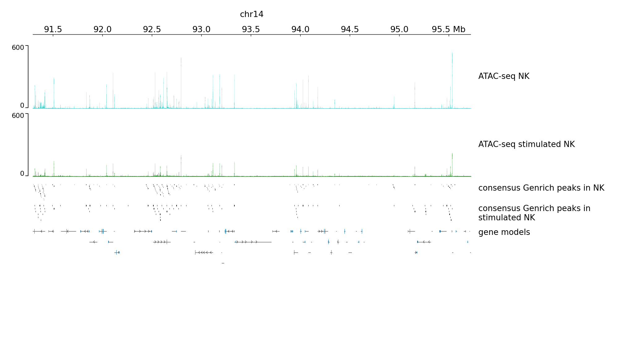
We can plot much wider region using these new settings:
pyGenomeTracks --tracks tracks2.ini --region chr14:91295621-95725599 --trackLabelFraction 0.2 --dpi 130 -o plot3.png
plot3.png
And so on, until we are satisfied with the figure.
There are more files linked in your working directory, you can try to visualise some of them. Try to select other regions, too.
Important List of available colours can be found at https://matplotlib.org/stable/gallery/color/named_colors.html .