Differential Accessibility in ATAC-seq

Learning outcomes

to perform GC-aware normalisation of ATAC-seq data using EDASeq
to detect differentially accessible regions using edgeR

Introduction 

In this tutorial we use an R / Bioconductor packages EDAseq and edgeR to perform normalisation and analysis of differential accessibility in ATAC-seq data.

Data & Methods 

We will build upon the main lab ATACseq data analysis:

first we will summarise reads to detected peaks using subset data as an example to obtain a counts table;
we will use the counts table encompassing complete data for differential accessibility analysis;

Setting-up 

We need access to file nk_merged_peaks.saf which we created in the ATACseq data analysis, part “Merged Peaks” and bam files with alignments.

Assuming we start at atacseq/analysis:

mkdir counts_table
cd counts_table

ln -s ../peaks/consensus/nk_merged_peaks.saf
ln -s ../../data_proc/* .

If you haven’t followed the peak calling and merging lab, you can continue from this point by linking necessary files:

ln -s ../../results/peaks/consensus/nk_merged_peaks.saf
ln -s ../../data_proc/* .

Data Summarisation 

We can now summarise the reads allowing for 20% overlap of the read length with peak feature (--fracOverlap 0.2) and counting fragments rather than reads (-p for PE):

module load subread/2.0.0
featureCounts -p -F SAF -a nk_merged_peaks.saf --fracOverlap 0.2 -o nk_merged_peaks_macs3.counts ENCFF363HBZ.chr14.proc.bam ENCFF398QLV.chr14.proc.bam ENCFF828ZPN.chr14.proc.bam ENCFF045OAB.chr14.proc.bam

Let’s take a look inside the counts table using head nk_merged_peaks_macs3.counts.

nk_merged_peaks_macs3.counts

head nk_merged_peaks_macs3.counts
# Program:featureCounts v2.0.0; Command:"featureCounts" "-p" "-F" "SAF" "-a" "nk_merged_peaks.saf" "--fracOverlap" "0.2" "-o" "nk_merged_peaks_macs3.counts" "ENCFF363HBZ.chr14.proc.bam" "ENCFF398QLV.chr14.proc.bam" "ENCFF828ZPN.chr14.proc.bam" "ENCFF045OAB.chr14.proc.bam"
Geneid  Chr     Start   End     Strand  Length  ENCFF363HBZ.chr14.proc.bam      ENCFF398QLV.chr14.proc.bam      ENCFF828ZPN.chr14.proc.bam      ENCFF045OAB.chr14.proc.bam
nk_merged_macs3_1       chr14   19161216        19161474        .       259     12      8       36      16
nk_merged_macs3_2       chr14   19161804        19162012        .       209     9       6       45      32
nk_merged_macs3_3       chr14   19239901        19240289        .       389     22      18      64      38
nk_merged_macs3_4       chr14   19384255        19384509        .       255     3       11      35      27
nk_merged_macs3_5       chr14   19488513        19488925        .       413     26      17      95      71
nk_merged_macs3_6       chr14   20305439        20306101        .       663     339     372     143     97
nk_merged_macs3_7       chr14   20332839        20333570        .       732     262     228     199     135
nk_merged_macs3_8       chr14   20342750        20343788        .       1039    2555    2424    1774    1226

We should remove the first line starting with #, as it can interfere with the way R reads in data:

awk '(NR>1)' nk_merged_peaks_macs3.counts > nk_merged_peaks_macs3.counts.tsv

Differential Accessibility 

Please note that in the following exercise we use a counts table generated using a different peak set, hence some small differences to peaks called during the course may be present.

You can continue working in the atacseq/analysis/counts directory. This directory contains merged peaks called earlier using macs3 callpeak as well as count tables derived from summarising of non-subset data (we won’t need the count tables for this exercise). We will use file nk_merged_peaks_macs3.counts and annotation libraries, which are preinstalled. We access them via a module R_packages.

We now load R and packages:

module load R_packages/4.1.1

We activate R console upon typing R in the terminal.

We begin by loading necessary libraries:

library(edgeR)
library(EDASeq)

library(GenomicAlignments)
library(GenomicFeatures)

library(TxDb.Hsapiens.UCSC.hg38.knownGene)
library(wesanderson)

library(Hmisc)
library(dplyr)

txdb = TxDb.Hsapiens.UCSC.hg38.knownGene

ff = FaFile("/proj/epi2023/atacseq_proc/hg38ucsc/hg38.fa")

We can read in the data, format it and define experimental groups:

cnt_table = read.table("nk_merged_peaks_macs3.counts", sep="\t", header=TRUE, blank.lines.skip=TRUE)
rownames(cnt_table)=cnt_table$Geneid

#update colnames of this count table
colnames(cnt_table)=c("Geneid","Chr","Start","End","Strand","Length","ENCFF363HBZ","ENCFF398QLV","ENCFF045OAB","ENCFF828ZPN")


groups = factor(c(rep("NK",2),rep("NKstim",2)))

#this data frame contains only read counts to peaks on assembled chromosomes
reads.peak = cnt_table[,c(7:10)]

We now prepare data with GC content of the peak regions for GC-aware normalisation.

gr = GRanges(seqnames=cnt_table$Chr, ranges=IRanges(cnt_table$Start, cnt_table$End), strand="*", mcols=data.frame(peakID=cnt_table$Geneid))

peakSeqs = getSeq(x=ff, gr)

gcContentPeaks = letterFrequency(peakSeqs, "GC",as.prob=TRUE)[,1]

#divide into 20 bins by GC content
gcGroups = Hmisc::cut2(gcContentPeaks, g=20)
mcols(gr)$gc = gcContentPeaks

Figure below shows that the accessibility measure of a particular genomic region is associated with its GC content. However, the slope and shape of the curves may differ between samples, which indicates that GC content effects are sample–specific and can therefore bias between–sample comparisons.

To visualise GC bias in peaks:

lowListGC = list()
for(kk in 1:ncol(reads.peak)){
  set.seed(kk)
  lowListGC[[kk]] = lowess(x=gcContentPeaks, y=log1p(reads.peak[,kk]), f=1/10)
}

names(lowListGC)=colnames(reads.peak)

dfList = list()
for(ss in 1:length(lowListGC)){
  oox = order(lowListGC[[ss]]$x)
  dfList[[ss]] = data.frame(x=lowListGC[[ss]]$x[oox], y=lowListGC[[ss]]$y[oox], sample=names(lowListGC)[[ss]])
}
dfAll = do.call(rbind, dfList)
dfAll$sample = factor(dfAll$sample)

p1.1 = ggplot(dfAll, aes(x=x, y=y, group=sample, color=sample)) +
  geom_line(size = 1) +
  xlab("GC-content") +
  ylab("log(count + 1)") +
  theme_classic()

pdf("GCcontent_peaks.pdf")
## plot just the average GC content
p1.1
dev.off()

Counts vs GC contents in ATAC-seq peaks.

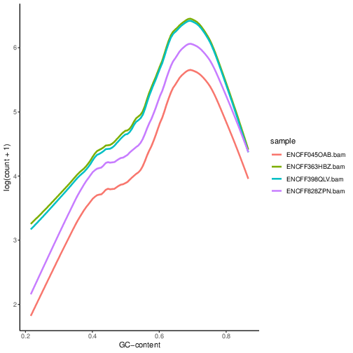
We can see that GC content has an effect on counts within the peaks.

We have seen from analyses presented on lecture slides and in https://www.biorxiv.org/content/10.1101/2021.01.26.428252v2 that full quantile normalisation (FQ-FQ) implemented in package EDASeq is one of the methods which can mitigate the GC bias in detection of DA regions.

We’ll detect differentially accessible regions using edgeR. We will input the normalised GC content as an offset to edgeR.

To calculate the offsets, which correct for library size as well as GC content (full quantile normalisation in both cases):

reads.peak=as.matrix(reads.peak)

dataOffset = withinLaneNormalization(reads.peak,y=gcContentPeaks,num.bins=20,which="full",offset=TRUE)
dataOffset = betweenLaneNormalization(reads.peak,which="full",offset=TRUE)

We now use the statistical framework of edgeR. We do not perform the internal normalisation (TMM) as usually, and instead we provide the offsets calculated by EDASeq.

design = model.matrix(~groups)

d = DGEList(counts=reads.peak, group=groups)

keep = filterByExpr(d)

> summary(keep)
        Mode   FALSE    TRUE
logical      21   54743


d=d[keep,,keep.lib.sizes=FALSE]

d$offset = -dataOffset[keep,]
d.eda = estimateGLMCommonDisp(d, design = design)
d.eda = estimateGLMCommonDisp(d, design = design)
fit = glmFit(d.eda, design = design)
lrt.EDASeq = glmLRT(fit, coef = 2)

DA_res=as.data.frame(topTags(lrt.EDASeq, nrow(lrt.EDASeq$table)))

The top DA peaks in stimulated vs non-stimulated NK cells:

> head(DA_res)

                         logFC   logCPM       LR       PValue          FDR
nk_merged_macs3_30535  6.404743 5.289554 442.7384 2.744592e-98 2.274389e-93
nk_merged_macs3_14734  6.403253 4.939915 432.3314 5.052034e-96 2.093260e-91
nk_merged_macs3_16907  6.199114 4.881266 415.2994 2.573898e-92 7.109792e-88
nk_merged_macs3_43844  7.262906 4.361125 398.6341 1.092157e-88 2.262621e-84
nk_merged_macs3_18163  5.626103 6.097144 397.4212 2.005906e-88 3.324509e-84
nk_merged_macs3_46357 -5.894601 5.021572 392.9164 1.918571e-87 2.649803e-83

Let’s add more peak information:

DA_res$Geneid = rownames(DA_res)
DA.res.coords = left_join(DA_res,cnt_table[1:4],by="Geneid")

        > head(DA.res.coords)
      logFC   logCPM       LR       PValue          FDR                Geneid
6.404743 5.289554 442.7384 2.744592e-98 2.274389e-93 nk_merged_macs3_30535
6.403253 4.939915 432.3314 5.052034e-96 2.093260e-91 nk_merged_macs3_14734
6.199114 4.881266 415.2994 2.573898e-92 7.109792e-88 nk_merged_macs3_16907
7.262906 4.361125 398.6341 1.092157e-88 2.262621e-84 nk_merged_macs3_43844
5.626103 6.097144 397.4212 2.005906e-88 3.324509e-84 nk_merged_macs3_18163
-5.894601 5.021572 392.9164 1.918571e-87 2.649803e-83 nk_merged_macs3_46357
    Chr     Start       End
chr17    642297    643906
chr11  86292675  86294054
chr12  24838503  24839731
chr2 157477051 157477910
chr12  68155671  68157629
chr2 241985117 241985981

We can now save the results:

write.table(DA.res.coords, "nk_DA_stim_vs_ctrl.tsv", quote = FALSE, sep = "\t",
    eol = "\n", na = "NA", dec = ".", row.names = FALSE,
    col.names = TRUE, fileEncoding = "")

We can check how well the GC correction worked:

gcGroups.sub=gcGroups[keep]
dfEdgeR = data.frame(logFC=log(2^lrt.EDASeq$table$logFC), gc=gcGroups.sub)

pedgeR = ggplot(dfEdgeR) +
  aes(x=gc, y=logFC, color=gc) +
  geom_violin() +
  geom_boxplot(width=0.1) +
  scale_color_manual(values=wesanderson::wes_palette("Zissou1", nlevels(gcGroups), "continuous")) +
  geom_abline(intercept = 0, slope = 0, col="black", lty=2) +
  ylim(c(-1,1)) +
  ggtitle("log2FCs in bins by GC content, FQ-FQ normalisation") +
  xlab("GC-content bin") +
  theme_bw()+
  theme(aspect.ratio = 1)+
  theme(axis.text.x = element_text(angle = 45, vjust = .5),
        legend.position = "none",
        axis.title = element_text(size=16))

ggsave(filename="log2FC_vs_GCcontent.EDAseq.pdf",plot=pedgeR ,path=".",device="pdf")

Dependence of log2FC on GC content in ATAC-seq.

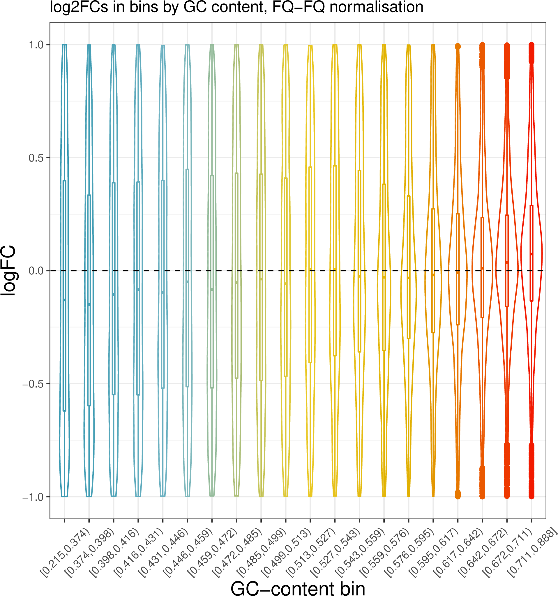
../../../_images/log2FC_vs_GCcontent.EDAseq.png

It seems that FQ-FQ normalisation did not completely remove the effect of GC content on log2FC in thie dataset. However, these effects are somewhat mitigated, you can compare this plot to one obtained by using the standard TMM normalisation.

Dependence of log2FC on GC content in ATAC-seq in non-GC corrected data.

d = DGEList(counts=reads.peak, group=groups)
keep = filterByExpr(d)
d=d[keep,,keep.lib.sizes=FALSE]
d = calcNormFactors(d)
#subset GRanges object for logFC binning
gr.sub=gr[keep,]
gcGroups.sub=gcGroups[keep]
d = estimateDisp(d, design)
fit <- glmFit(d, design)
lrt.tmm <- glmLRT(fit)
dfEdgeR = data.frame(logFC=log(2^lrt.tmm$table$logFC), gc=gcGroups.sub)


pedgeR <- ggplot(dfEdgeR) +
        aes(x=gc, y=logFC, color=gc) +
        geom_violin() +
         geom_boxplot(width=0.1) +
        theme_bw()+ theme(aspect.ratio = 1)+
        scale_color_manual(values=wesanderson::wes_palette("Zissou1", nlevels(gcGroups), "continuous")) +
        geom_abline(intercept = 0, slope = 0, col="black", lty=2) +
         ylim(c(-1,1)) +
         ggtitle("log2FCs in bins by GC content, TMM normalisation") +
         theme(axis.text.x = element_text(angle = 45, vjust = .5),
legend.position = "none",
axis.title = element_text(size=16))

ggsave(filename="log2FC_vs_GCcontent.TMM.pdf",plot=pedgeR ,path=".",device="pdf")

../../../_images/log2FC_vs_GCcontent.TMM.png

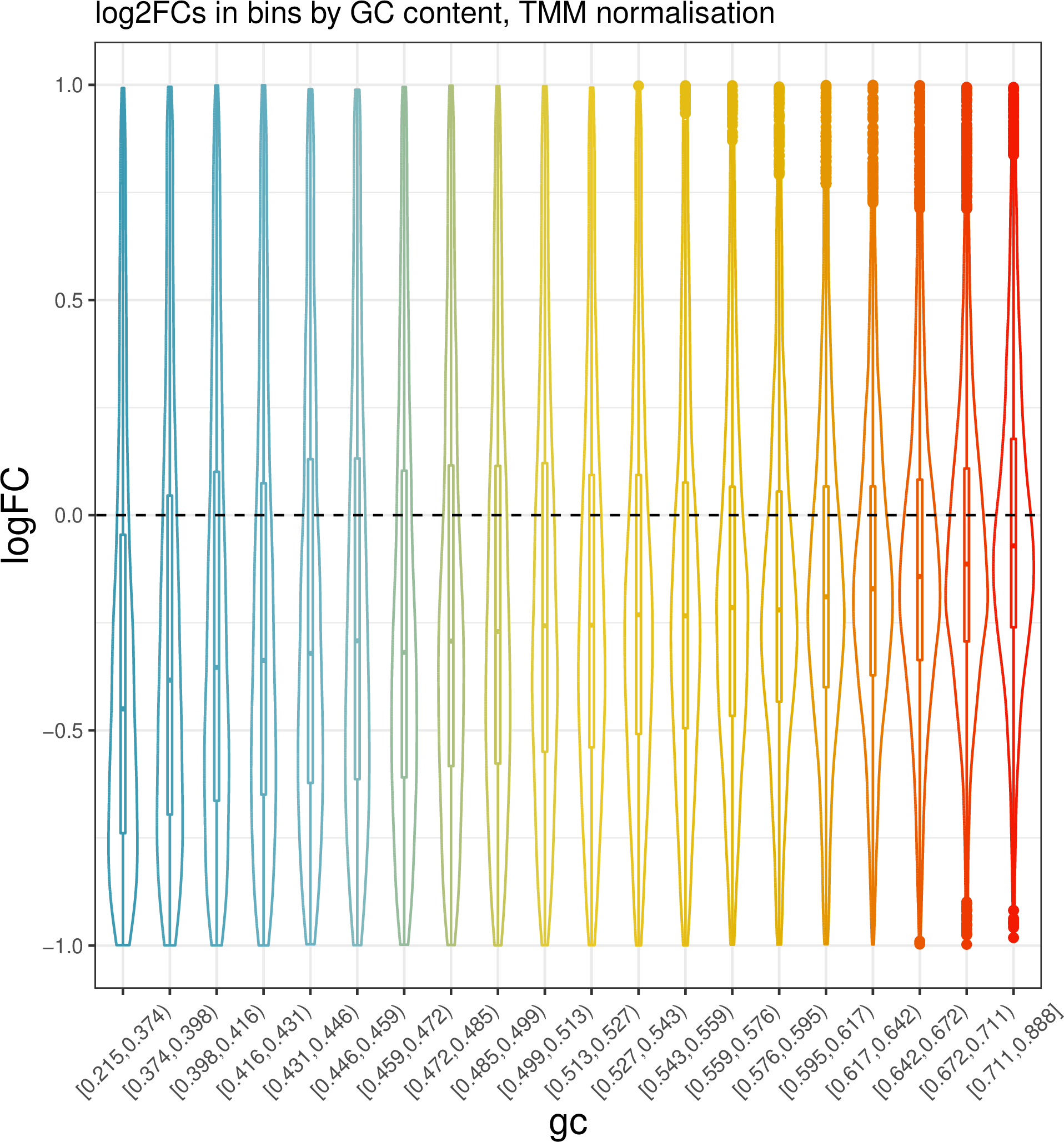
Part of the reason why the GC effects are not completely removed in this case may be that the fold change calculation/ DA analysis is not performed on properly replicated data; we should have at least 3 replicates per condition, and we only have two.

Differential Accessibility in ATAC-seq

Introduction

Data & Methods

Setting-up

Data Summarisation

Differential Accessibility

Introduction 

Data & Methods 

Setting-up 

Data Summarisation 

Differential Accessibility 