ChIP-seq down-stream analysis
Please note this tutorial is more than 4 years old. It uses older tools versions and has not been recently tested.
Learning outcomes
obtain differentially bound sites with
DiffBindannotate differentially bound sites with nearest genes and genomic features with
ChIPpeakAnnoperform functional enrichment analysis to identify predominant biological themes with
ChIPpeakAnnoandreactome.db
Introduction
In the previous tutorials we have learnt how to access the quality of ChIP-seq data and we how to derive a consensus peakset for downstream analyses.
In this part we will learn how to place the peaks in a biological context, by identifying differentially bound sites between two sample groups and annotating these sites to find out predominant biological themes separating the groups.
Data & Methods
We will continue using the same data as in the ChIP data processing and peak detection tutorial. Please note that usually three biological replicates are the minimum requirement for statistical analysis such as in factor occupancy.
Hint
The ENCODE data we are using have only two replicates and we are using them to demonstrate the tools and methodologies. No biological conclusions should be drawn from them, or as a matter of fact, from any other dataset with duplicates only. Just because the tool computes the results does not make it right!
Setting-up
The setting-up is the same as for the data processing tutorial, described in detail in section “Setting up directory structure and files”.
If you have logged out: log back in, open interactive session, and run chipseq_env.sh script.
If you followed the ChIP-seq Data Processing QC and Peak Calling lab, you can continue in chipseq/analysis/R.
If you haven’t, starting in your home directory, you need to copy data:
    cp /proj/epi2025/chipseq/scripts/chipseq_data.sh .
    bash chipseq_data.sh

cd chipseq/analysis/R
Differential binding
Intro
We will usage Bioconductor package DiffBind to identify sites that are differentially occupied between two sample groups.
The package includes “functions to support the processing of peak sets, including overlapping and merging peak sets, counting sequencing reads overlapping intervals in peak sets, and identifying statistically significantly differentially bound sites based on evidence of binding affinity (measured by differences in read densities). To this end it uses statistical routines developed in an RNA-Seq context (primarily the Bioconductor packages edgeR and DESeq2). Additionally, the package builds on Rgraphics routines to provide a set of standardized plots to aid in binding analysis.”
This means that we will repeat deriving a consensus peakset in a more powerful way before identifying differentially bound sites. Actually, identifying the consensus peaks is an important step that takes up entire chapter in the DiffBind manual. We recommend reading the section: 6_2 Deriving consensus peaksets.
So how does the differential binding affinity analysis work?
“The core functionality of DiffBind is the differential binding affinity analysis, which enables binding sites to be identified that are statistically significantly differentially bound between sample groups. To accomplish this, first a contrast (or contrasts) is established, dividing the samples into groups to be compared. Next the core analysis routines are executed, by default using DESeq2. This will assign a p-value and FDR to each candidate binding site indicating confidence that they are differentially bound.”
Setting-up DiffBind
Let’s
- load R packges module that has a bunch of R packages, including DiffBind package, installed on Uppmax.
- go to the right directory given you are keeping files structure as for the first part of the tutorial.
Hint
If you start from a different location, you should cd ~/chipseq/analysis/R
In this directory we have placed a sample sheet file named samples_REST.txt that points to our BAM files as well as BED files with called peaks, following DiffBind specifications, and as created in data processing tutorial. To inspect sample sheet file:
head samples_REST.txt
You can now load the version of R for which we tested this class along with other dependencies:
module load R_packages/4.0.4
The remaining part of the exercise is performed in R.
Hint
We are running
R version 4.0.4 (2021-02-15) -- "Lost Library Book"
Let’s open R on Uppmax by simply typing R
R
From within R we need to load DiffBind library
library(DiffBind)
Running DiffBind
We will now follow DiffBind example to obtain differentially bound sites in our samples (several cell lines). You may want to open DiffBind tutorial and read section 3 Example Obtaining differentially bound sites while typing the command to get more information about each step.
First we need to create the object which holds data.
# reading in the sample information (metadata)
samples = read.csv("samples_REST.txt", sep="\t")

# inspecting the metadata
samples

# creating an object containing data
res=dba(sampleSheet=samples, config=data.frame(RunParallel=TRUE))

# inspecting the object: how many peaks are identified given the default settings?
res
res
   8 Samples, 6518 sites in matrix (17056 total):
          ID Tissue Factor Replicate Intervals
1 REST_chip1   HeLa   REST         1      2252
2 REST_chip2   HeLa   REST         2      2344
3 REST_chip3 neural   REST         1      5948
4 REST_chip4 neural   REST         2      3003
5 REST_chip5  HepG2   REST         1      2663
6 REST_chip6  HepG2   REST         2      4326
7 REST_chip7  sknsh   REST         1      8700
8 REST_chip8  sknsh   REST         2      3524
Let’s continue with the analysis. The wrapper function dba.count reads in data.
# counting reads mapping to intervals (peaks)
res.cnt = dba.count(res, minOverlap=2, score=DBA_SCORE_TMM_MINUS_FULL, fragmentSize=130)

# applying  TMM normalisation
res.norm=dba.normalize(res.cnt, normalize=DBA_NORM_TMM)

# inspecting the object: notice the FRiP values!
res.norm
res.norm
> res.norm
     8 Samples, 6389 sites in matrix:
               ID Tissue Factor Replicate   Reads FRiP
     1 REST_chip1   HeLa   REST         1 1637778 0.10
     2 REST_chip2   HeLa   REST         2 1991560 0.07
     3 REST_chip3 neural   REST         1 3197782 0.05
     4 REST_chip4 neural   REST         2 4924672 0.06
     5 REST_chip5  HepG2   REST         1 2988915 0.05
     6 REST_chip6  HepG2   REST         2 4812034 0.05
     7 REST_chip7  sknsh   REST         1 2714033 0.09
     8 REST_chip8  sknsh   REST         2 4180463 0.05
To inspect the normalisation factors:
dba.normalize(res.norm, bRetrieve=TRUE)
We will set the contrasts to test:
# setting the contrast
res.cnt2 = dba.contrast(res.cnt, categories=DBA_TISSUE, minMembers=2)

# inspecting the object: how many contrasts were set in the previous step
res.cnt2
These are the contrasts we can test:
 res.cnt2
8 Samples, 6389 sites in matrix:
          ID Tissue Factor Replicate   Reads FRiP
1 REST_chip1   HeLa   REST         1 1637778 0.10
2 REST_chip2   HeLa   REST         2 1991560 0.07
3 REST_chip3 neural   REST         1 3197782 0.05
4 REST_chip4 neural   REST         2 4924672 0.06
5 REST_chip5  HepG2   REST         1 2988915 0.05
6 REST_chip6  HepG2   REST         2 4812034 0.05
7 REST_chip7  sknsh   REST         1 2714033 0.09
8 REST_chip8  sknsh   REST         2 4180463 0.05

Design: [~Tissue] | 6 Contrasts:
  Factor  Group Samples Group2 Samples2
1 Tissue   HeLa       2 neural        2
2 Tissue   HeLa       2  HepG2        2
3 Tissue   HeLa       2  sknsh        2
4 Tissue neural       2  HepG2        2
5 Tissue neural       2  sknsh        2
6 Tissue  sknsh       2  HepG2        2
We can save some plots of data exploration, to copy to your local computer and view later:
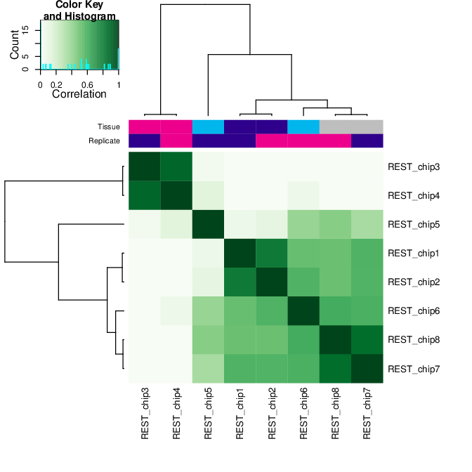
# plotting the correlation of libraries based on normalised counts of reads in peaks
pdf("correlation_libraries_normalised.pdf")
plot(res.cnt)
dev.off()
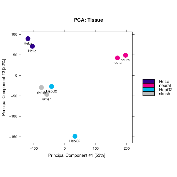
# PCA scores plot: data overview
pdf("PCA_normalised_libraries.pdf")
dba.plotPCA(res.cnt,DBA_TISSUE,label=DBA_TISSUE)
dev.off()
correlation_libraries_normalised.pdf
PCA_normalised_libraries.pd
The analysis of differential occupancy is performed by a wrapper function dba.analyze. You can adjust the settings using variables from the DBA class, for details consult DiffBind User Guide and DiffBind manual .
# we will skip generating greylists (regions of high signal in input samples) because of time - it is recommended to perform this step in your own analyses though!
res.cnt2$config$doGreylist=FALSE

# performing analysis of differential binding
res.cnt3 = dba.analyze(res.cnt2)

# inspecting the object: which condition are most alike, which are most different, is this expected?
dba.show(res.cnt3, bContrasts = T)
The res.cnt3 object:
>dba.show(res.cnt3, bContrasts = T)
  Factor  Group Samples Group2 Samples2 DB.DESeq2
1 Tissue   HeLa       2 neural        2      2559
2 Tissue   HeLa       2  HepG2        2       912
3 Tissue   HeLa       2  sknsh        2       365
4 Tissue neural       2  HepG2        2      1916
5 Tissue neural       2  sknsh        2      2561
6 Tissue  sknsh       2  HepG2        2       348
We can save some more of many useful plots implemented in DiffBind:
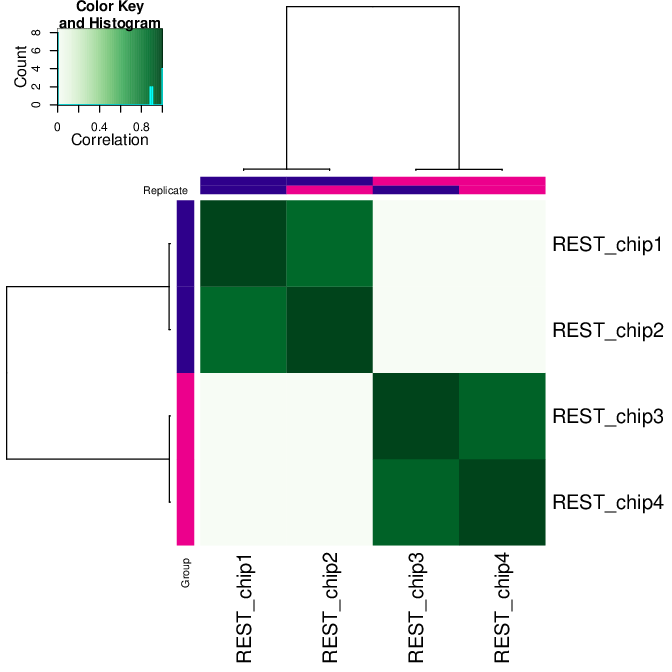
# correlation heatmap using only significantly differentially bound sites
# choose the contrast of interest e.g. HeLa vs. neuronal (#1)
pdf("correlation_HeLa_vs_neuronal.pdf")
plot(res.cnt3, contrast=1)
dev.off()
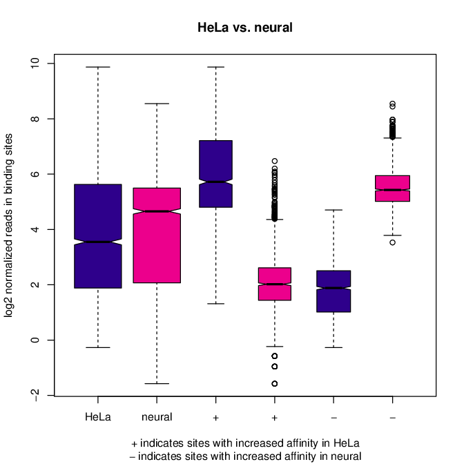
# boxplots to view how read distributions differ between classes of binding sites
# are reads distributed evenly between those that increase binding affinity HeLa vs. in neuronal?
pdf("Boxplot_HeLa_vs_neuronal.pdf")
pvals <- dba.plotBox(res.cnt3, contrast=1)
dev.off()
correlation_HeLa_vs_neuronal.pdf
Boxplot_HeLa_vs_neuronal.pdf
Finally, we can save the results, for HeLa vs neural cells:
# extracting differentially occupied sites in a GRanges object
res.db1 = dba.report(res.cnt3, contrast=1)
head(res.db1)
res.db1 contains:
GRanges object with 6 ranges and 6 metadata columns:
       seqnames              ranges strand |      Conc Conc_HeLa Conc_neural
          <Rle>           <IRanges>  <Rle> | <numeric> <numeric>   <numeric>
  1175     chr1   64808799-64809199      * |   7.06770   8.06046    0.425017
  2617     chr1 200466043-200466443      * |   7.17091   8.17091    0.000000
  2729     chr1 204378226-204378626      * |   6.26091   7.26091    0.000000
  2353     chr1 171282842-171283242      * |   6.17060   7.13789    1.691067
   917     chr1   44997690-44998090      * |   7.03490   8.03490    0.000000
   783     chr1   38331405-38331805      * |   6.99800   7.99318    0.000000
            Fold     p-value         FDR
       <numeric>   <numeric>   <numeric>
  1175   6.79730 4.55123e-09 1.16113e-05
  2617   9.00133 5.00132e-09 1.16113e-05
  2729   8.46198 6.13580e-09 1.16113e-05
  2353   5.15165 7.27071e-09 1.16113e-05
   917   8.86864 9.49523e-09 1.21311e-05
   783   7.32153 1.23421e-08 1.27646e-05
  -------
  seqinfo: 2 sequences from an unspecified genome; no seqlengths
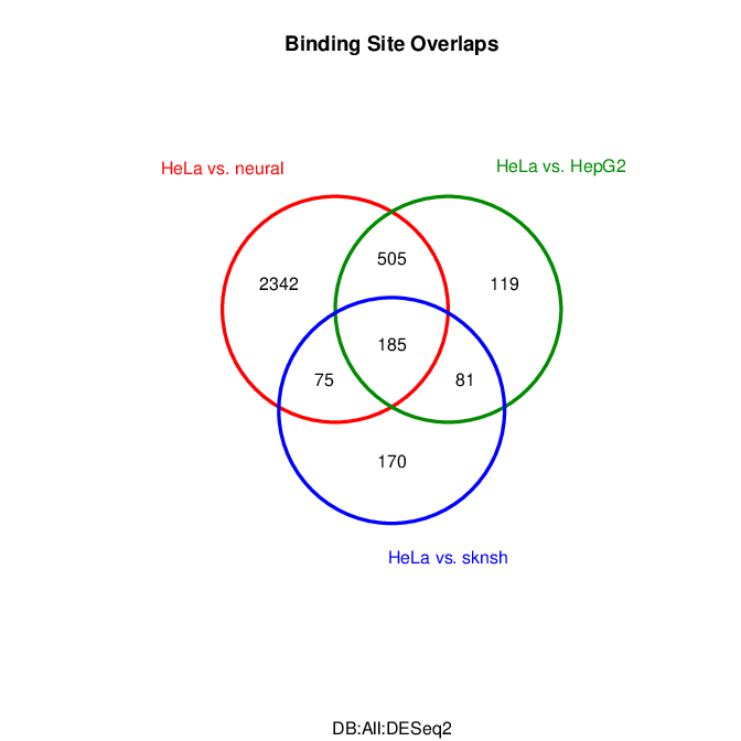
Results summary in a Venn diagram:
# plotting overlaps of sites bound by REST in different cell types
pdf("binding_site_overlap.pdf")
dba.plotVenn(res.cnt3, contrast=c(1:3))
dev.off()
binding_site_overlap.pdf
Save the session:
# finally, let's save our R session including the generated data. We will need everything in the next section
save.image("diffBind.RData")
relevant information from sessionInfo()
other attached packages:
 [1] DiffBind_3.0.15             SummarizedExperiment_1.20.0
 [3] Biobase_2.50.0              MatrixGenerics_1.2.1
 [5] matrixStats_0.58.0          GenomicRanges_1.42.0
 [7] GenomeInfoDb_1.26.7         IRanges_2.24.1
 [9] S4Vectors_0.28.1            BiocGenerics_0.36.0
Appendix: figures
Fig: Correlation of libraries based on normalised counts of reads in peaks
Fig: PCA scores plot: data overview using normalised counts of reads in peaks
Fig: Correlation heatmap using only significantly differentially bound sites for HeLa and neuronal
Fig: Boxplots of reads distributions between HeLa and neuronal
Fig: Venn diagram of overlapping sites bound by REST in different cell types