Detection of broad peaks from ChIP-seq data

Learning outcomes

• be able to assess the quality of ChIP-seq data for factors with broad occupancy pattern

• be able to detect regions of enrichment for factors with broad occupancy pattern

Requirements

• MACS 3.0.0a6

• epic2 0.0.52

• R version 4.0.4 (2021-02-15) -- "Lost Library Book"

• csaw 1.24.3 and its dependencies

Bioconductor packages required for annotation:

• org.Hs.eg.db

• TxDb.Hsapiens.UCSC.hg38.knownGene

For details please consult Dependencies.

Please note that this lab consists of three parts:

1. calling broad peaks using MACS (Uppmax);

2. calling broad peaks using epic2 (Uppmax); and

3. finding enriched genomic windows using csaw in R (Uppmax / local).

Notes on software

We provide a conda environment to run epic2. This package proved a bit tricky to install because of dependency incompatibilities. To find how this environment was constructed, please visit Dependencies.

Please note that this workflow has been tested using R 4.0.4 and csaw 1.24.3 on Uppmax only.

Data

We will use ChIP-seq of H3K79me2 from ENCODE. H3K79me2 is enriched at active promoters and linked to transcriptional activation as it tends to accumulate in transcribed regions of active genes.

The samples are from GM23338 cell line (human induced pluripotent stem cell from skin fibroblasts) before and after stimulation with doxycycline to form bipolar neurons.

These data are paired-end with read length 76 bp (2x76) and consist of duplicates of H3K79me2 ChIP and matching input samples. Raw data was processed using ENCODE3 pipeline and mapped to GRCh38 genome assembly. We have further processed the data to remove unwanted signal and subset to chromosomes 1 and 2, as in the tutorial ChIPseq data processing. Accession details are summarised in Table 1.

Table 1. Samples and accessions in the data set used in this exercise.

Sample	ENCODE Accession	Replicate
GM23338, H3K79me2 ChIP	ENCFF263XBT	rep 1
GM23338, H3K79me2 ChIP	ENCFF531WSU	rep 2
GM23338, input	ENCFF992ZBS	rep 1
GM23338, input	ENCFF237PRF	rep 2
neuro GM23338, H3K79me2 ChIP	ENCFF395DAJ	rep 1
neuro GM23338, H3K79me2 ChIP	ENCFF806KRA	rep 2
neuro GM23338, input	ENCFF956GLJ	rep 1
neuro GM23338, input	ENCFF687LIL	rep 2

We will detect occupancy regions from one sample only, and compare the results to other samples processed earlier.

Quality control

As always, one should start the analysis from assesment of data quality. This is already performed to save time, and the plots and metrics are included below.

Cross-correlation and related metrics

The files discussed in this section can be accessed at /proj/epi2023/broad_peaks/results/qc

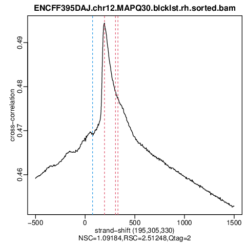
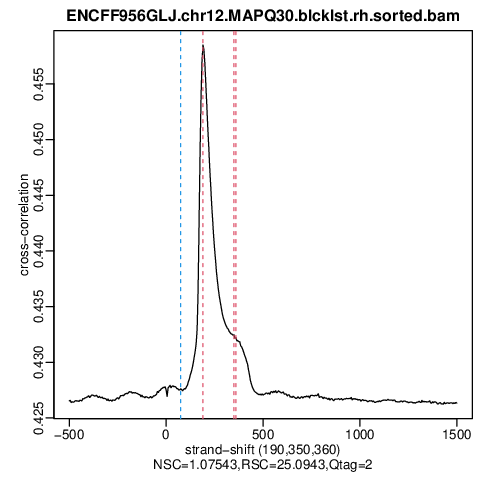
These metrics have been developed with application to point source (i.e. TFs and narrow histone modifications) ChIP-seq in mind, and you can see that the results for broad domains are not as easy to interpret as for point source factors. Below are cross correlation plots for the IP and input you are going to use for the exercise.

Already from these plots alone it is evident that the data has some quality issues. At this point you should be able to identify them.

Figure 1. Cross correlations in H3K79me2 ChIP and input samples in GM23338-derived neuron cells (ENCODE).

K79me2 ChIP (ENCFF395DAJ)	input (ENCFF956GLJ)

The cross correlation profile of factors with broad occupancy patterns is not going to be as sharp as for TFs, and the values of NSC and RSC tend to be lower, which does not mean that the ChIP failed. In fact, the developers of the tool do not recommend using the same NSC / RSC values as quality cutoffs for broad marks. However, input samples should not display signs of enrichment, as is the case here.

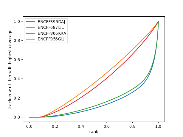
Cumulative enrichment

Another plot worth examining is cumulative enrichment (aka fingerprint from deepTools):

Figure 2. Cumulative enrichment (bamFingerprint) in H3K79me2 ChIP and input samples in GM23338-derived neuron cells (ENCODE).

all samples

You can see that even though the cross correlation metrics don’t look great, a significant enrichment can be observed for the ChIP samples (ENCFF395DAJ, ENCFF806KRA), and not for the input samples.

Broad peak calling using MACS

MACS: Model-based Analysis for ChIP-Seq is one of the leading peak calling algorithms. We will use MACS version 3, which is still under active development and hasn’t been officially released.

You will call peaks using sample GM23338 neuro - H3K79me2 ChIP ENCFF395DAJ and its matching input ENCFF956GLJ.

Effective genome size for chr 1 and 2 in hg38 is 4.9e8.

mkdir -p analysis/macs3
cd analysis/macs3

ln -s /proj/epi2023/broad_peaks/data/neuron_GM23338/ENCFF395DAJ.chr12.MAPQ30.blcklst.rh.sorted.bam
ln -s /proj/epi2023/broad_peaks/data/neuron_GM23338//ENCFF956GLJ.chr12.MAPQ30.blcklst.rh.sorted.bam

module load bioinfo-tools #if needed
module load MACS/3.0.0a6

macs3 callpeak --broad \
-t ENCFF395DAJ.chr12.MAPQ30.blcklst.rh.sorted.bam \
-c ENCFF956GLJ.chr12.MAPQ30.blcklst.rh.sorted.bam \
-f BAMPE  -g 04.9e8 --broad-cutoff 0.1 -n neuroGM23338_macs3_rep1

The main difference here, in comparison to detecting narrow peaks, is using the options --broad --broad-cutoff 0.1. With the option --broad on, MACS will try to composite broad regions in BED12 (gene-model-like format) by putting nearby highly enriched regions into a broad region with loose cutoff. The broad region is controlled by another cutoff through --broad-cutoff. If -p is set, this is a p-value cutoff, otherwise, it’s a q-value (FDR) cutoff.

Because we use PE data, there is no need to build a model to estimate fragment length (similar to cross correlation) necessary for extending the SE reads. We know precisely how long each fragment is because its both ends are sequenced and mapped to the reference. Estimating fragment length from cross-correlation of broad domain ChIP data is problematic and sometimes may result in incorrect values.

You can now inspect the results in the output folder macs3. The structure is alike the output for calling narrow peaks. The file *.broadPeak is in BED6+3 format which is similar to narrowPeak file used for point-source factors, except for missing the 10th column for annotating peak summits. Look at MACS repository homepage for details.

The meaning of columns in NAME_peaks.xls files:

chr

chromosome name

start

start position of peak

end

end position of peak

length

length of peak region

pileup

pileup height at peak summit

-log10(pvalue)

-log10(pvalue) for the peak summit (e.g. pvalue =1e-10, then this value should be 10)

fold_enrichment

fold enrichment for this peak summit against random Poisson distribution with local lambda

-log10(qvalue)

-log10(qvalue) at peak summit

name

peak id

Let’s take a look at another format of the output broadPeak. It is a derivative of bed format and thus compatible with major genome browsers (IGV, UCSC Genome Browser) and easier to work with because it does not contain a long header.

This is an example:

head neuroGM23338_macs3_rep1_peaks.broadPeak

chr1  777491  778262  neuroGM23338_macs3_rep1_peak_1  34  . 3.542 4.93525 3.48401
chr1  779812  780867  neuroGM23338_macs3_rep1_peak_2  10  . 2.28884 2.27839 1.03252
chr1  782000  784521  neuroGM23338_macs3_rep1_peak_3  17  . 2.6654  3.01765 1.70342
chr1  820548  826643  neuroGM23338_macs3_rep1_peak_4  36  . 3.5486  5.10182 3.65624
chr1  828271  830128  neuroGM23338_macs3_rep1_peak_5  34  . 3.4958  4.87316 3.42798
chr1  831350  833671  neuroGM23338_macs3_rep1_peak_6  22  . 2.7518  3.55309 2.20097
chr1  882552  890194  neuroGM23338_macs3_rep1_peak_7  34  . 3.21783 4.86863 3.43262
chr1  925794  926897  neuroGM23338_macs3_rep1_peak_8  18  . 2.71963 3.12803 1.80546
chr1  957085  959246  neuroGM23338_macs3_rep1_peak_9  60  . 4.54986 7.61848 6.03443
chr1  999291  999914  neuroGM23338_macs3_rep1_peak_10 16  . 2.63811 2.95948 1.65064

The meaning of columns in NAME.broadPeak files:

chrom

Name of the chromosome (or contig, scaffold, etc.).

chromStart

The starting position of the feature in the chromosome or scaffold. The first base in a chromosome is numbered 0.

chromEnd

The ending position of the feature in the chromosome or scaffold. The chromEnd base is not included in the display of the feature. For example, the first 100 bases of a chromosome are defined as chromStart=0, chromEnd=100, and span the bases numbered 0-99. If all scores were “0” when the data were submitted to the DCC, the DCC assigned scores 1-1000 based on signal value. Ideally the average signalValue per base spread is between 100-1000.

name

Name given to a region (preferably unique). Use “.” if no name is assigned.

score

Indicates how dark the peak will be displayed in the browser (0-1000).

strand

+/- to denote strand or orientation (whenever applicable). Use “.” if no orientation is assigned.

signalValue

Measurement of overall (usually, average) enrichment for the region.

pvalue

Measurement of statistical significance (-log10). Use -1 if no pValue is assigned.

qValue

Measurement of statistical significance using false discovery rate (-log10). Use -1 if no qValue is assigned.

How many peaks were identified in replicate 1?

wc -l neuroGM23338_macs3_rep1_peaks.broadPeak
6826 neuroGM23338_macs3_rep1_peaks.broadPeak

Hint

You can also copy the results from /proj/epi2023/broad_peaks/results/macs3/neuroGM23338

This is a preliminary peak list, and in case of broad domains, it often needs some processing or filtering.

Let’s select the detected domains reproducible in both replicates. First, let’s create a subdirectory peaks, and link the results of broad peak calling. Then we select the first 6 columns of broadPeak to create files in BED-6 format, which are ready for use by bedtools. After completing the tutorial on data processing you should be able to find the peaks reproducible between the replicates. How many of them can we identify?

mkdir peaks
cd peaks
ln -s /proj/epi2023/broad_peaks/results/macs3/neuroGM23338/neuroGM23338_macs3_rep1_peaks.broadPeak
ln -s /proj/epi2023/broad_peaks/results/macs3/neuroGM23338/neuroGM23338_macs3_rep2_peaks.broadPeak

#make bed
cut -f 1-6 neuroGM23338_macs3_rep1_peaks.broadPeak >neuroGM23338_macs3_rep1_peaks.bed
cut -f 1-6 neuroGM23338_macs3_rep2_peaks.broadPeak >neuroGM23338_macs3_rep2_peaks.bed

Select reproducible peaks (MACS).

#intersect bed files
module load bioinfo-tools #if needed
module load BEDTools/2.29.2
bedtools intersect -a neuroGM23338_macs3_rep1_peaks.bed -b neuroGM23338_macs3_rep2_peaks.bed -f 0.50 -r > peaks_macs3_neuroGM23338.chr12.bed

#how many peaks which overlap?
wc -l peaks_macs3_neuroGM23338.chr12.bed
2679 peaks_macs3_neuroGM23338.chr12.bed

Visual inspection of the peaks (MACS)

You will use IGV for this step, and it is recommended that you run it locally on your own computer. Please load hg38 reference genome.

Required files are:

• ChIP ENCFF395DAJ.chr12.MAPQ30.blcklst.rh.sorted.bam and matching bai

• input ENCFF956GLJ.chr12.MAPQ30.blcklst.rh.sorted.bam and matching bai

• signal domains neuroGM23338_macs3_rep1_peaks.broadPeak

• reproducible signal domains peaks_macs3_neuroGM23338.chr12.bed

Hint

You can access the bam and bai files from /proj/epi2023/broad_peaks/data/neuron_GM23338

You can look at some locations of interest. Peaks with low FDR (q value) or high fold enrichment may be worth checking out. We find these peaks by numerically sorting the results in broadPeak by column “score” (the 5th column). Or check your favourite gene.

Potentially interesting locations to view (MACS peaks).

Let’s sort the broadPeak file using the score column to find the peaks with the strongest signal

sort -k5,5rn neuroGM23338_macs3_rep1_peaks.broadPeak | head

chr1 226062814 226073870 neuroGM23338_macs3_rep1_peak_3341 518 . 13.0292 54.709  51.8498
chr1  234598782 234610959 neuroGM23338_macs3_rep1_peak_3515 513 . 12.139  54.2276 51.3993
chr2  101698297 101748719 neuroGM23338_macs3_rep1_peak_5147 462 . 13.375  49.0116 46.2392
chr2  47158830  47176361  neuroGM23338_macs3_rep1_peak_4479 449 . 12.5555 47.6423 44.96
chr1  204403186 204412701 neuroGM23338_macs3_rep1_peak_2999 431 . 10.9654 45.8227 43.1784
chr1  220527779 220538029 neuroGM23338_macs3_rep1_peak_3239 414 . 11.5724 44.1237 41.4922
chr1  244049535 244060201 neuroGM23338_macs3_rep1_peak_3688 403 . 10.2749 42.9757 40.397
chr2  54970096  55050304  neuroGM23338_macs3_rep1_peak_4577 401 . 11.3781 42.7092 40.1167
chr2  5692693 5703228 neuroGM23338_macs3_rep1_peak_3837 399 . 10.6746 42.502  39.9488
chr1  150568640 150579241 neuroGM23338_macs3_rep1_peak_2121 394 . 11.0116 42.0139 39.4717

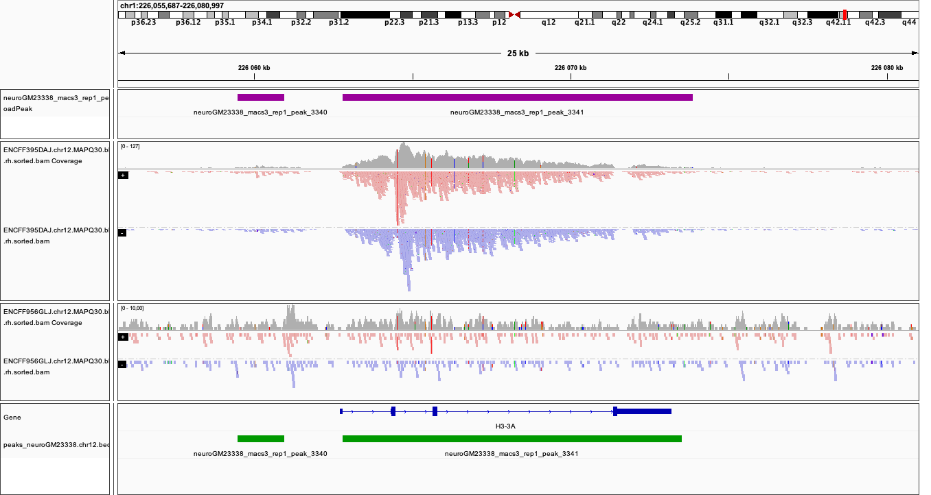
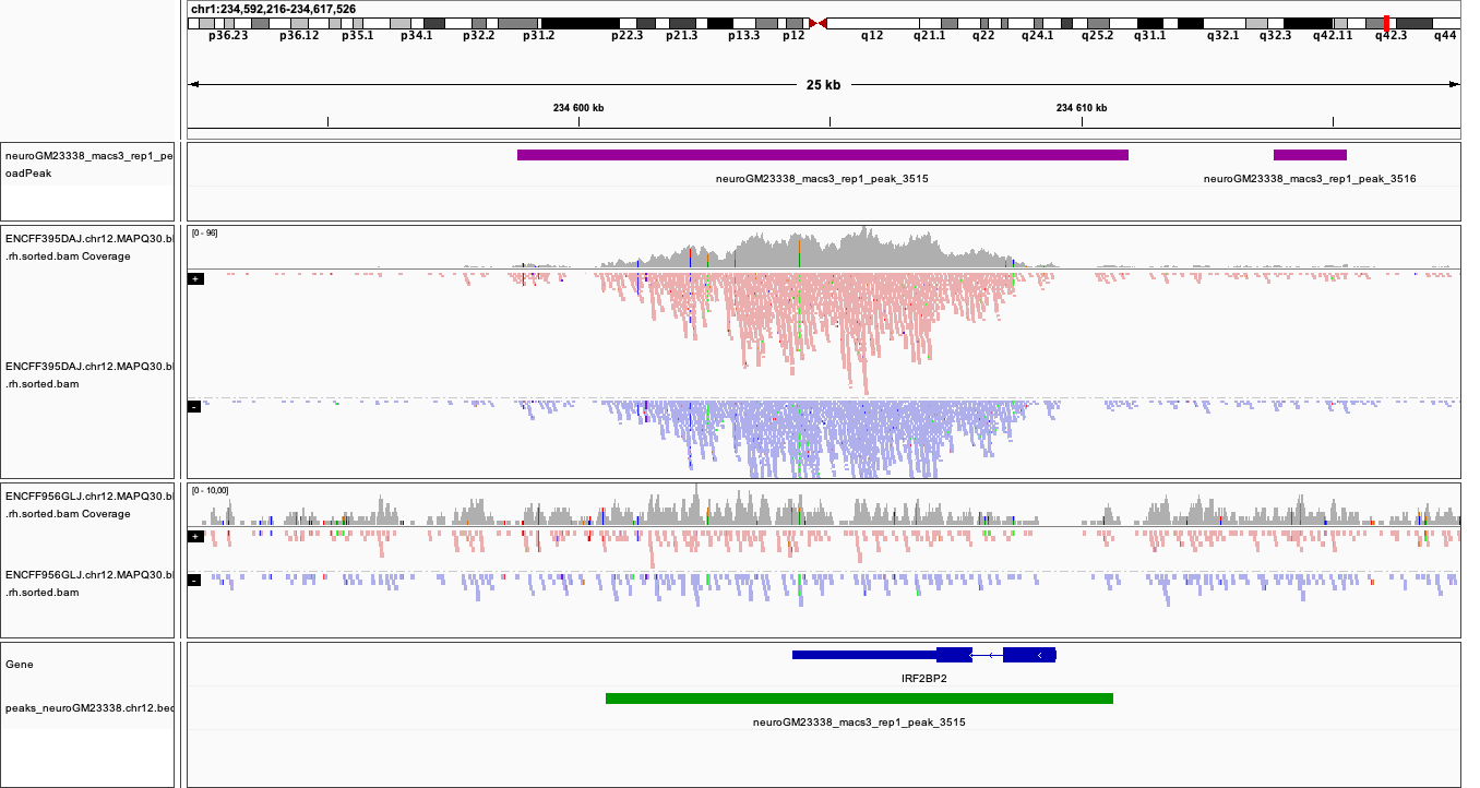
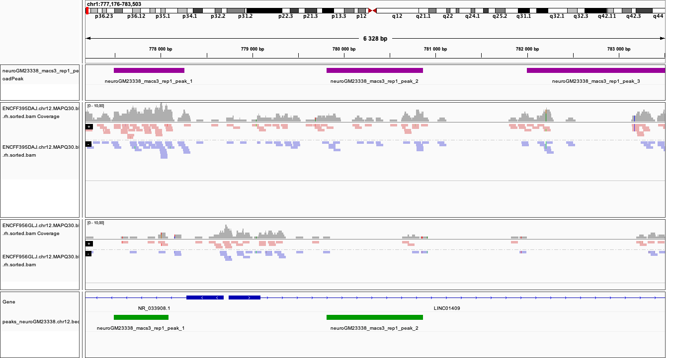
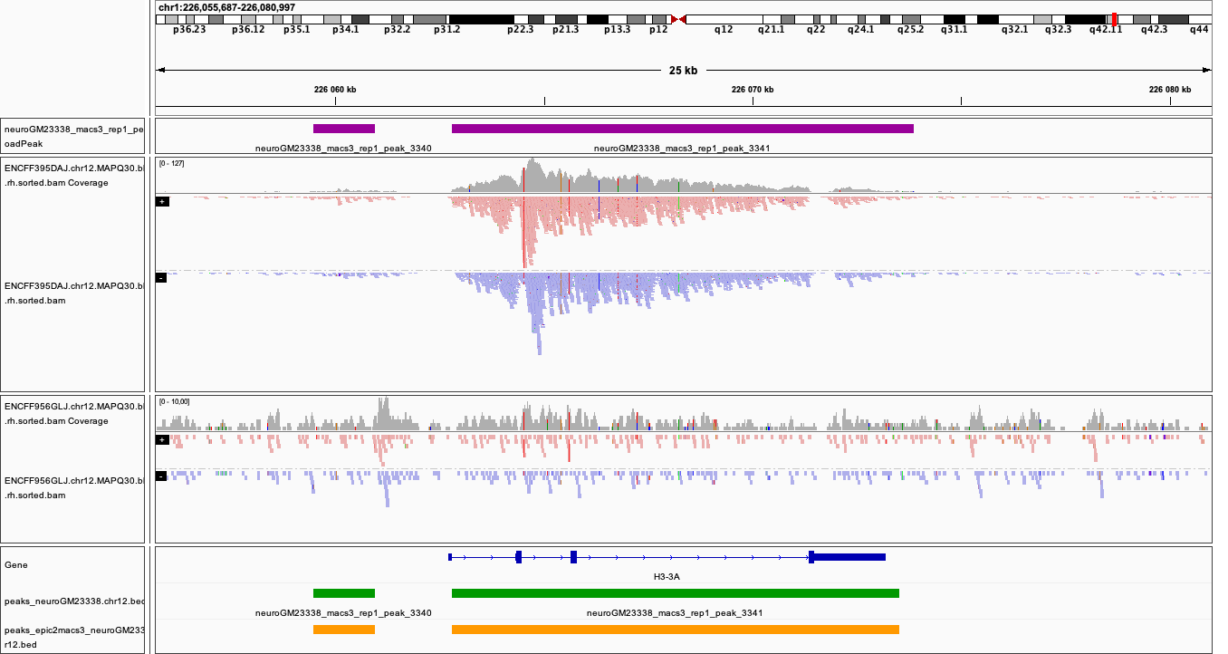
Below you see IGV visualisations of the following regions (top two peaks and one of the bottom rank):

chr1:226,055,687-226,080,997
chr1:234,592,216-234,617,526
chr1:777,176-783,503

IGV settings for this visualiation (right click on the left hand side panel with track names): Group alignments (by read strand); Colour alignments (by read strand); Squished.

Regions detected by MACS3 are the topmost purple track, two bam files are ChIP and input (with their pileups calculated by IGV), and the bottom panel are gene models and, finally the regions reproducible between both replicates in green.

Please note the length of these detected domains.

Figure 3. Results of peak calling in H3K79me2 ChIP-seq in GM23338-derived neuron cells (ENCODE). Tracks from the top: peaks in rep1, ChIP, input, gene models, reproducible peaks

Broad peak calling using epic2

epic2 is an ultraperformant reimplementation of SICER, an algorithm developed especially for detection of broad marks. It focuses on speed, low memory overhead and ease of use. It also contains a reimplementation of the SICER-df scripts for differential enrichment and a script to create many kinds of bigwigs from your data. In this tutorial we will use it to detect domains in the same data as we used earlier for MACS. At the end we will compare the results.

Here again we use a prepared conda environment. Newer versions of Pysam seem to throw errors when used with epic2. For details please consult Dependencies.

mkdir ../../epic2
cd ../../epic2

ln -s /proj/epi2023/broad_peaks/data/neuron_GM23338/ENCFF395DAJ.chr12.MAPQ30.blcklst.rh.sorted.bam
ln -s /proj/epi2023/broad_peaks/data/neuron_GM23338/ENCFF395DAJ.chr12.MAPQ30.blcklst.rh.sorted.bam.bai
ln -s /proj/epi2023/broad_peaks/data/neuron_GM23338//ENCFF956GLJ.chr12.MAPQ30.blcklst.rh.sorted.bam
ln -s /proj/epi2023/broad_peaks/data/neuron_GM23338//ENCFF956GLJ.chr12.MAPQ30.blcklst.rh.sorted.bam.bai


conda activate /sw/courses/epigenomics/software/conda/epic_2b

epic2 --treatment ENCFF395DAJ.chr12.MAPQ30.blcklst.rh.sorted.bam \
 --control ENCFF956GLJ.chr12.MAPQ30.blcklst.rh.sorted.bam \
  -fdr 0.05 --effective-genome-fraction 0.95 \
  --chromsizes /sw/courses/epigenomics/broad_peaks2/annot/hg38_chr12.chromsizes \
  --guess-bampe --output neuroGM23338_epic2_rep1_peaks

The result is a coordinate sorted text file:

head neuroGM23338_epic2_rep1_peaks
#Chromosome Start End PValue  Score Strand  ChIPCount InputCount  FDR log2FoldChange
chr1  777400  778199  1.525521715195486e-17 302.351431362403  . 28  4 3.6469084588658344e-17  3.02351431362403
chr1  821600  822599  9.82375064925635e-15  309.0628509482567 . 22  3 2.149649196967778e-14 3.090628509482567
chr1  823400  826599  1.912606813336636e-50 258.96177870938703  . 114 22  7.16207410279741e-50  2.58961778709387
chr1  828200  830399  5.824989404621774e-19 201.13395996779278  . 59  17  1.4498521203360967e-18  2.0113395996779277
chr1  831400  833599  2.388427396703667e-14 151.73289262869903  . 69  28  5.17334134771682e-14  1.5173289262869905
chr1  880600  885799  2.569723734705377e-37 153.80874864537878  . 195 78  8.520333236155976e-37 1.538087486453788
chr1  886600  890199  1.481460204837024e-22 165.05622157122005  . 100 37  3.9835062883707675e-22  1.6505622157122006
chr1  925800  926999  8.491192455372113e-17 280.11218922875815  . 30  5 1.9845609170824598e-16  2.801121892287582
chr1  957000  959199  4.1356938759907084e-64  337.1437617044337 . 98  11  1.688095302270476e-63 3.3714376170443368

The meaning of the columns:

PValue

Poisson-computed PValue based on the number of ChIP count vs. library-size normalized Input count in the region

Score

Log2FC * 100 (capped at 1000). Regions with a larger relative ChIP vs. Input count will show as darker in the UCSC genome browser

ChIPCount

The number of ChIP counts in the region (also including counts from windows with a count below the cutoff)

InputCount

The number of Input counts in the region

FDR

Benjamini-Hochberg correction of the p-values

log2FoldChange

Log2 of the region ChIP count vs. the library-size corrected region Input count

How many domains were found? (the first line is a header)

wc -l neuroGM23338_epic2_rep1_peaks
5242 neuroGM23338.rep1.epic2

How many domains reproducible between replicates?

Select reproducible peaks (epic2).

mkdir peaks
cd peaks

#link the files
ln -s /sw/courses/epigenomics/broad_peaks2021/results/epic2/neuroGM23338/neuroGM23338.rep1.epic2
ln -s /sw/courses/epigenomics/broad_peaks2021/results/epic2/neuroGM23338/neuroGM23338.rep2.epic2

#make bed
cut -f 1-3 neuroGM23338.rep1.epic2 >neuroGM23338_epic2_rep1_peaks.bed
cut -f 1-3 neuroGM23338.rep2.epic2 >neuroGM23338_epic2_rep2_peaks.bed

#intersect bed files
module load bioinfo-tools #if necessary
module load BEDTools/2.29.2
bedtools intersect -a neuroGM23338_epic2_rep1_peaks.bed -b neuroGM23338_epic2_rep2_peaks.bed -f 0.50 -r > peaks_epic2_neuroGM23338.chr12.bed

#how many peaks which overlap?
wc -l peaks_epic2_neuroGM23338.chr12.bed
2692 peaks_epic2_neuroGM23338.chr12.bed

How about the overlap between different methods?

Compare MACS3 and epic2.

(please make sure the relative path to macs3 results is correct in the command below)

#intersect bed files
module load bioinfo-tools #if necessary
module load BEDTools/2.29.2
bedtools intersect -a peaks_epic2_neuroGM23338.chr12.bed -b ../../macs3/peaks/peaks_macs3_neuroGM23338.chr12.bed \
-f 0.50 -r > peaks_epic2macs3_neuroGM23338.chr12.bed

#how many peaks which overlap?
wc -l peaks_epic2macs3_neuroGM23338.chr12.bed
1629 peaks_epic2macs3_neuroGM23338.chr12.bed

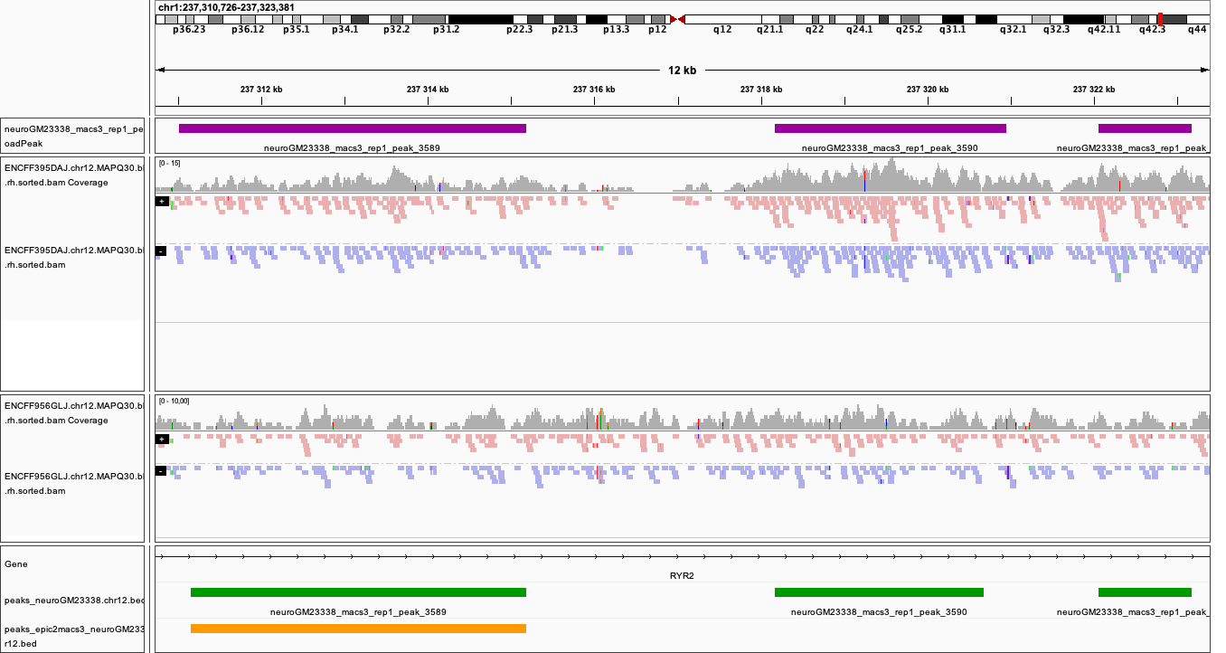
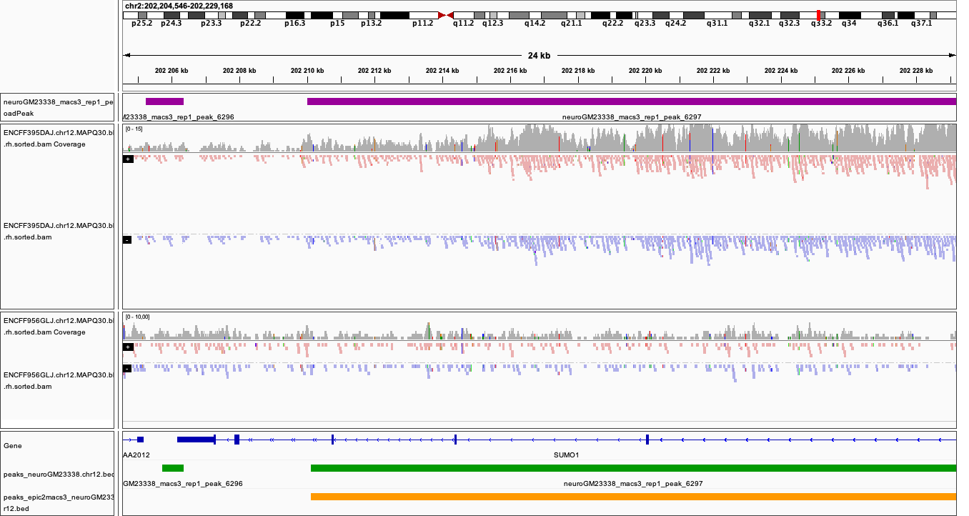
You can visualise the peaks as for MACS in the earlier section. Below are plots of some of the locations as in the MACS, with peaks detected by both epic2 and MACS marked in orange.

Figure 4. Results of peak calling in H3K79me2 ChIP-seq in GM23338-derived neuron cells (ENCODE). Comparison of MACS3 and epic2. Tracks from the top: peaks in rep1, ChIP, input, gene models, reproducible peaks (MACS3), peaks detected by epic2 and MACS3 (orange)

Locations plotted.

chr1:226,055,687-226,080,997
chr1:237,310,726-237,323,381
chr2:202,204,546-202,229,168

You can now deactivate the conda environment you’ve been working in:

conda deactivate

Alternative approach: window-based enrichment analysis (csaw)

This is an alternative workflow for detection of differential binding / occupancy in ChIP-seq data. In this mode, in contrast to working with reads counted within peaks detected in a peak calling step (as in the earlier example with DiffBind), this approach uses a sliding window to count reads across the genome. Each window is then tested for significant differences between libraries from different conditions, using the methods in the edgeR package. This package also offers an FDR control strategy more appropriate for ChIP-seq experiments than simple BH adjustment. csaw can also be used to detect peaks - if the sample to compare to is input.

As this method is agnostic to signal structure, it requires careful choice of strategies for filtering and normalisation. Here, we show a very simple workflow. More details can be found in the Csaw User Guide.

Note

This exercise was tested on Rackham using pre-installed R libraries. Local installation of recommended R packages may require additional software dependecies. Please see Dependencies for details.

Requirements Remote (Uppmax)

The software is configured, i.e. the correct R version is loaded via the module system and required libraries are preinstalled.

To prepare the files, assuming you are in ~/broad_peaks/analysis:

mkdir csaw
cd csaw

mkdir bam
ln -s  /proj/epi2023/broad_peaks/data/neuron_GM23338/* bam

module load R_packages/4.0.4

The remaining part of the exercise is performed in R.

Sort out the working directory and file paths:

setwd("/path/to/workdir")

dir.data = "/path/to/desired/location/bam"

#for example when in broad_peaks/csaw
dir.data = "./bam"

k79_1=file.path(dir.data,"ENCFF395DAJ.chr12.MAPQ30.blcklst.rh.sorted.bam")
input_1=file.path(dir.data,"ENCFF956GLJ.chr12.MAPQ30.blcklst.rh.sorted.bam")
k79_2=file.path(dir.data,"ENCFF806KRA.chr12.MAPQ30.blcklst.rh.sorted.bam")
input_2=file.path(dir.data,"ENCFF687LIL.chr12.MAPQ30.blcklst.rh.sorted.bam")

bam.files <- c(k79_1,k79_2,input_1,input_2)

Hint

Setting the paths in R

To find the path to your current location type pwd in the terminal. You can use this path in R like this:

setwd("/path/to/where_you_are")

All the paths will be then relative to /path/to/where_you_are.

You can also find it directly from R using getwd:

> getwd()
[1] "/crex/course_data/epigenomics/broad_peaks2021/results/csaw"

Read in the data:

library(csaw)

pe.param <- readParam(max.frag=400, pe="both")
data <- windowCounts(bam.files, width=100, param=pe.param)

ChIP experiments with paired-end sequencing are accomodated by setting pe="both" in the param object supplied to windowCounts. Read extension is not required as the genomic interval spanned by the originating fragment is explicitly defined as that between the 5′positions of the paired reads. By default, only proper pairs are used in which the two paired reads are on the same chromosome, face inward and are no more than max.frag apart (we use the default value 500, which is suitable for most libraries). width specifies the width of the window when counting the fragments.

How many valid windows do we have?:

data$totals
[1]  3666329  5635840  4436456 16125939

data

> data
 class: RangedSummarizedExperiment
 dim: 8808414 4
 metadata(6): spacing width ... param final.ext
 assays(1): counts
 rownames: NULL
 rowData names(0):
 colnames: NULL
 colData names(4): bam.files totals ext rlen

You will identify the enrichment windows by performing a differential occupancy analysis between ChIP and input samples.

Information on the contrast to test:

grouping <- factor(c('chip', 'chip', 'input', 'input'))
design <- model.matrix(~0 + grouping)
colnames(design) <- levels(grouping)
library(edgeR)
contrast <- makeContrasts(chip - input, levels=design)

contrast

> contrast
 Contrasts
Levels  chip - input
  chip             1
  input           -1

Next, you need to filter out uninformative windows with low signal prior to further analysis. Selection of appropriate filtering strategy and cutoff is key to a successful detection of differential occupancy events, and is data dependent. Filtering is valid so long as it is independent of the test statistic under the null hypothesis. One possible approach involves choosing a filter threshold based on the fold change over the level of non-specific enrichment (background). The degree of background enrichment is estimated by counting reads in large bins across the genome.

The function filterWindowsGlobal returns the increase in the abundance of each window over the global background. Windows are filtered by setting some minimum threshold on this increase. Here, a fold change of 3 is necessary for a window to be considered as containing a binding site. This and other filtering procedures are described in detail in csaw user guide . We use the “By global enrichment” strategy.

In this example, you estimate the global background using ChIP samples only. You can do it using the entire dataset including inputs of course.

bam.files_chip <- c(k79_1,k79_2)

bin.size <- 2000L
binned.ip <- windowCounts(bam.files_chip, bin=TRUE, width=bin.size, param=pe.param)
data.ip=data[,1:2]
filter.stat <- filterWindowsGlobal(data.ip, background=binned.ip)

keep <- filter.stat$filter > log2(3)
data.filt <- data[keep,]

To examine how many windows passed the filtering:

      summary(keep)
       Mode   FALSE    TRUE
logical 7466311  731112

To normalise the data for different library sizes you need to calculate normalisation factors based on large bins:

binned <- windowCounts(bam.files, bin=TRUE, width=10000, param=pe.param)
data.filt <- normFactors(binned, se.out=data.filt)

data.filt$norm.factors
## [1] 0.6094691 0.6654708 1.5651132 1.5753374

Detection of DB (differentially bound) windows (in our case, the occupancy sites, as we test for differences in ChIP vs. input):

data.filt.calc <- asDGEList(data.filt)
data.filt.calc <- estimateDisp(data.filt.calc, design)
fit <- glmQLFit(data.filt.calc, design, robust=TRUE)
results <- glmQLFTest(fit, contrast=contrast)

You can inspect the raw results:

head(results$table)
   logFC    logCPM        F       PValue
1 4.397419 0.1113531 39.71585 1.054723e-07
2 3.957880 0.1781093 36.54985 2.550295e-07
3 4.079911 0.2803444 42.31232 5.243527e-08
4 3.920461 0.4808799 47.20246 1.487789e-08
5 4.410081 0.5664205 59.33251 8.606713e-10
6 5.026440 0.6390274 69.96147 9.239046e-11

The following steps will calculate the FDR for each peak, merge peaks within 1 kb and calculate the FDR for resulting composite peaks.

merged <- mergeWindows(rowRanges(data.filt), tol=1000L)
table.combined <- combineTests(merged$id, results$table)

Short inspection of the results:

head(table.combined)

DataFrame with 6 rows and 8 columns
  num.tests num.up.logFC num.down.logFC      PValue         FDR   direction
  <integer>    <integer>      <integer>   <numeric>   <numeric> <character>
1        12           12              0 1.10869e-09 6.83746e-09          up
2         9            9              0 5.54991e-06 1.53993e-05          up
3        54           54              0 1.28669e-10 9.16836e-10          up
4        29           29              0 3.25906e-08 1.59822e-07          up
5        36           36              0 3.14755e-07 1.26463e-06          up
6         1            1              0 1.06514e-05 2.62040e-05          up
   rep.test rep.logFC
  <integer> <numeric>
1         6   5.02644
2        14   4.11686
3        61   4.42842
4        85   3.70258
5       113   3.45417
6       141   3.45264

How many regions are up (i.e. enriched in chip compared to input)?

is.sig.region <- table.combined$FDR <= 0.1
table(table.combined$direction[is.sig.region])

  up
  8116

Does this make sense? How does it compare to results obtained from MACS and epic2 runs?

You can now annotate the results:

library(org.Hs.eg.db)
library(TxDb.Hsapiens.UCSC.hg38.knownGene)

anno <- detailRanges(merged$region, txdb=TxDb.Hsapiens.UCSC.hg38.knownGene,
orgdb=org.Hs.eg.db, promoter=c(3000, 1000), dist=5000)

merged$region$overlap <- anno$overlap
merged$region$left <- anno$left
merged$region$right <- anno$right

all.results <- data.frame(as.data.frame(merged$region)[,1:3], table.combined, anno)

sig=all.results[all.results$FDR<0.05,]
all.results <- all.results[order(all.results$PValue),]

head(all.results)

filename="k79me2_neuroGM_csaw.txt"
write.table(all.results,filename,sep="\t",quote=FALSE,row.names=FALSE)

Let’s inspect the results:

head(all.results)
      seqnames     start       end num.tests num.up.logFC num.down.logFC
3799     chr1 226062751 226073900       213          213              0
870      chr1  35176951  35193200       319          319              0
5154     chr2  47157601  47178000       344          344              0
4233     chr1 244835751 244867200       617          617              0
4003     chr1 234598601 234610800       211          211              0
2608     chr1 160363601 160374200       205          205              0
           PValue          FDR direction rep.test rep.logFC
3799 2.124641e-23 1.306798e-19        up   351746  6.758585
870  5.493232e-23 1.306798e-19        up    92252  7.177477
5154 6.358299e-23 1.306798e-19        up   459830  6.833969
4233 6.750822e-23 1.306798e-19        up   390369  6.430975
4003 8.050751e-23 1.306798e-19        up   369849  6.761304
2608 1.305657e-22 1.560297e-19        up   253600  6.381518
                    overlap         left right
3799   H3-3A:+:PE,H3P6:+:PE   H3P6:+:657
870  RNVU1-18:-:I,SFPQ:-:PE   SFPQ:-:477
5154  STPG4:-:PE,CALM2:-:PE STPG4:-:2293
4233 COX20:+:PE,HNRNPU:-:PE
4003           IRF2BP2:-:PE
2608             NHLH1:+:PE NCSTN:+:4649

To compare with peaks detected by MACS it is convenient to save the results in BED format:

sig.up=sig[sig$direction=="up",]

starts=sig.up[,2]-1

sig.up[,2]=starts

sig_bed=sig.up[,c(1,2,3)]

filename="k79me2_neuroGM_csaw_peaks.bed"
write.table(sig_bed,filename,sep="\t",col.names=FALSE,quote=FALSE,row.names=FALSE)

You can now load the bed file to IGV along with the appropriate broad.Peak file and zoom in to your favourite location on chromosomes 1 and 2.

Below is the IGV snapshot of top peak, this time with csaw peaks added in light blue.

Figure 5. Results of broad peak calling in H3K79me2 ChIP-seq in GM23338-derived neuron cells (ENCODE). Comparison of MACS3, epic2 and csaw. Tracks from the top: peaks in rep1, ChIP, input, gene models, reproducible peaks (MACS3), peaks detected by epic2 and MACS3 (orange), peaks deteced by csaw (light blue).

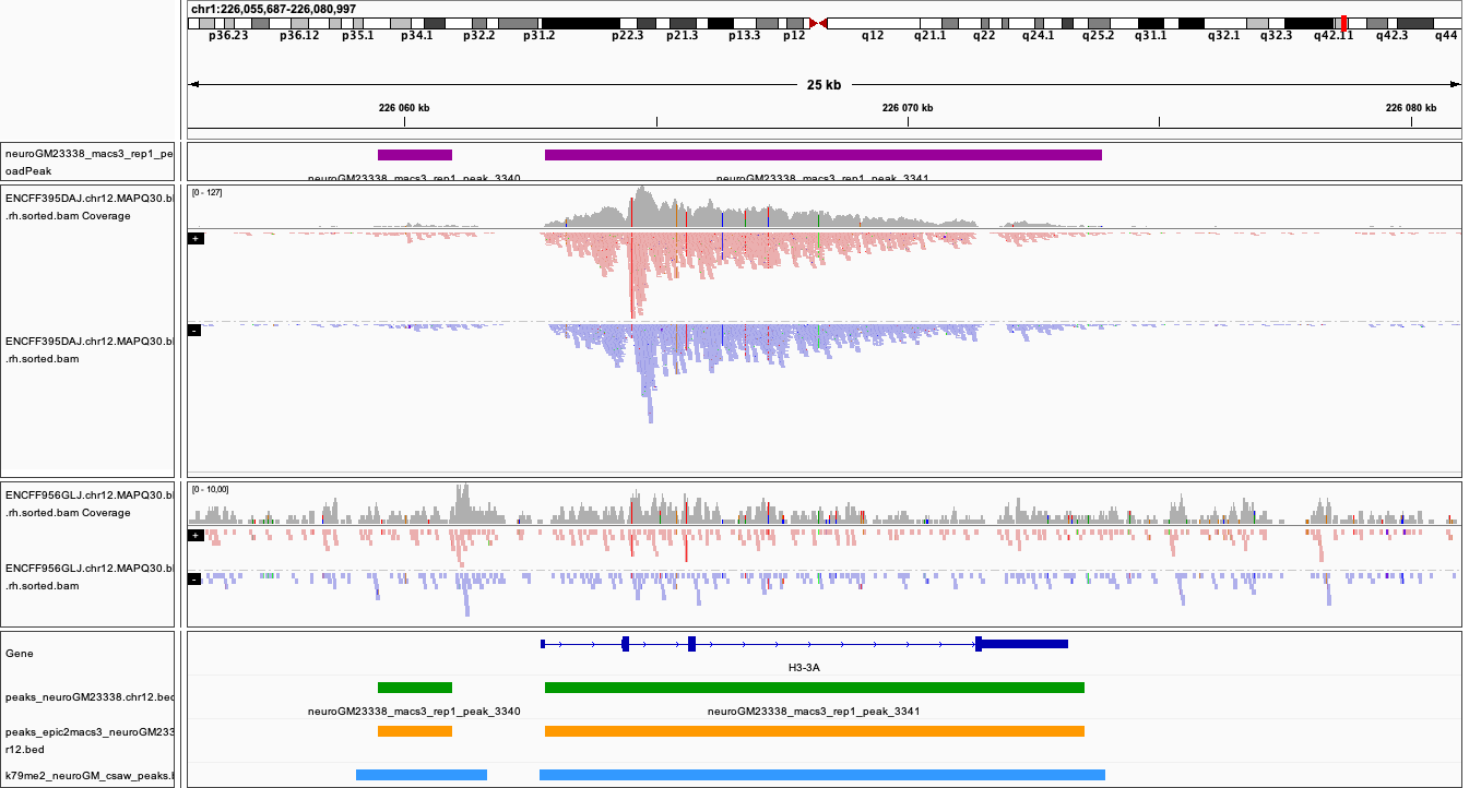
As you can see the regions with strong signal (high enrichment in ChIP over input) are detected by all methods tested. What about the sites with weak signal?

In this tutorial we have worked with good quality data which was sequenced to a recommended depth. All three methods tested in this tutorial perform well is such scenario. However, their preformace deteriorates with decreasing sequening depth (less data to rely on) and decreasing quality of the sample preparation (more noise).

sessionInfo()

 Random number generation:
 RNG:     Mersenne-Twister
 Normal:  Inversion
 Sample:  Rejection

attached base packages:
[1] parallel  stats4    stats     graphics  grDevices utils     datasets
[8] methods   base

other attached packages:
 [1] TxDb.Hsapiens.UCSC.hg38.knownGene_3.10.0
 [2] GenomicFeatures_1.42.3
 [3] org.Hs.eg.db_3.12.0
 [4] AnnotationDbi_1.52.0
 [5] edgeR_3.32.1
 [6] limma_3.46.0
 [7] csaw_1.24.3
 [8] SummarizedExperiment_1.20.0
 [9] Biobase_2.50.0
[10] MatrixGenerics_1.2.1
[11] matrixStats_0.58.0
[12] GenomicRanges_1.42.0
[13] GenomeInfoDb_1.26.7
[14] IRanges_2.24.1
[15] S4Vectors_0.28.1
[16] BiocGenerics_0.36.0

loaded via a namespace (and not attached):
 [1] locfit_1.5-9.4           Rcpp_1.0.6               lattice_0.20-41
 [4] Rsamtools_2.6.0          prettyunits_1.1.1        Biostrings_2.58.0
 [7] assertthat_0.2.1         utf8_1.2.1               BiocFileCache_1.14.0
[10] R6_2.5.0                 RSQLite_2.2.6            httr_1.4.2
[13] pillar_1.6.0             zlibbioc_1.36.0          rlang_0.4.10
[16] progress_1.2.2           curl_4.3                 rstudioapi_0.13
[19] blob_1.2.1               Matrix_1.3-2             splines_4.0.4
[22] statmod_1.4.35           BiocParallel_1.24.1      stringr_1.4.0
[25] RCurl_1.98-1.3           bit_4.0.4                biomaRt_2.46.3
[28] DelayedArray_0.16.3      compiler_4.0.4           rtracklayer_1.50.0
[31] pkgconfig_2.0.3          askpass_1.1              openssl_1.4.3
[34] tidyselect_1.1.0         tibble_3.1.1             GenomeInfoDbData_1.2.4
[37] XML_3.99-0.6             fansi_0.4.2              crayon_1.4.1
[40] dplyr_1.0.5              dbplyr_2.1.1             GenomicAlignments_1.26.0
[43] bitops_1.0-6             rappdirs_0.3.3           grid_4.0.4
[46] lifecycle_1.0.0          DBI_1.1.1                magrittr_2.0.1
[49] stringi_1.5.3            cachem_1.0.4             XVector_0.30.0
[52] xml2_1.3.2               ellipsis_0.3.1           vctrs_0.3.7
[55] generics_0.1.0           tools_4.0.4              bit64_4.0.5
[58] glue_1.4.2               purrr_0.3.4              hms_1.0.0
[61] fastmap_1.1.0            memoise_2.0.0