Peak Annotation
Learning outcomes
Using ChIPseeker package
to profile ATAC-seq signal by genomics location and by proximity to TSS regions
to annotate peaks with the nearest gene
to run and compare functional enrichment
Introduction
In this tutorial we use an R / Bioconductor package ChIPseeker, to have a look at the ATAC / ChIP profiles, annotate peaks and visualise annotations.
We will also perform functional annotation of peaks using clusterProfiler.
The tutorial is based on the ChIPseeker package tutorial so feel free to have this open alongside to read and experiment more.
Data & Methods
We will build upon the main labs:
ATAC-seq: all detected peaks (merged consensus peaks);
ATAC-seq: differentially accessible peaks;
Setting-up
You can continue working in the atacseq/analysis/counts directory. This directory contains merged peaks called earlier using macs3 callpeak as well as count tables derived from summarising of non-subset data (we won’t need the count tables for this exercise). We will use file nk_merged_peaksid.bed and annotation libraries, which are preinstalled. We access them via:
module load R_packages/4.1.1
We activate R console upon typing R in the terminal.
We begin by loading necessary libraries:
library(ChIPseeker)
library(TxDb.Hsapiens.UCSC.hg38.knownGene)

library(GenomicAlignments)
library(GenomicFeatures)

library(clusterProfiler)
library(biomaRt)
library(org.Hs.eg.db)
library(ReactomePA)

txdb <- TxDb.Hsapiens.UCSC.hg38.knownGene
Peaks Coverage Plot
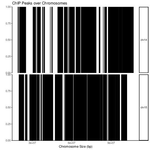
After peak calling one may want to visualise distribution of peaks locations over the whole genome. Function covplot calculates coverage of peaks regions over chromosomes.
Let’s load in the data (peaks called on nun subset data) and transform the data frame to GenomicRanges object (GRanges):
pth2peaks_bed="nk_merged_peaksid.bed"

peaks.bed=read.table(pth2peaks_bed, sep="\t", header=FALSE, blank.lines.skip=TRUE)
rownames(peaks.bed)=peaks.bed[,4]

peaks.gr <- GRanges(seqnames=peaks.bed[,1], ranges=IRanges(peaks.bed[,2], peaks.bed[,3]), strand="*", mcols=data.frame(peakID=peaks.bed[,4]))
If you are not familiar with GRanges objects, this is how the structure is:
GRanges object with 83180 ranges and 1 metadata column:
          seqnames              ranges strand |          mcols.peakID
             <Rle>           <IRanges>  <Rle> |           <character>
      [1]     chr1         10003-10442      * |     nk_merged_macs3_1
      [2]     chr1         28932-29454      * |     nk_merged_macs3_2
      [3]     chr1       180755-181134      * |     nk_merged_macs3_3
      [4]     chr1       181359-181895      * |     nk_merged_macs3_4
      [5]     chr1       183598-183831      * |     nk_merged_macs3_5
      ...      ...                 ...    ... .                   ...
  [83176]     chrX 155997332-155997955      * | nk_merged_macs3_83176
  [83177]     chrX 156016605-156016865      * | nk_merged_macs3_83177
  [83178]     chrX 156025043-156025495      * | nk_merged_macs3_83178
  [83179]     chrX 156028799-156029148      * | nk_merged_macs3_83179
  [83180]     chrX 156030182-156030752      * | nk_merged_macs3_83180
  -------
  seqinfo: 91 sequences from an unspecified genome; no seqlengths
To inspect peak coverage along the chromosomes:
covplot(peaks.gr, chrs=c("chr14", "chr15"))

#to save the image to file
pdf("PeakCoverage.pdf")
covplot(peaks.gr, chrs=c("chr14", "chr15"))
dev.off()
Distribution of ATAC peaks along chromosomes.
Peak Annotation
To annotate peaks with closest genomic features:
bed.annot = annotatePeak(peaks.gr, tssRegion=c(-3000, 3000),TxDb=txdb, annoDb="org.Hs.eg.db")
Let’s inspect the results:
> bed.annot
Annotated peaks generated by ChIPseeker
82916/83180  peaks were annotated
Genomic Annotation Summary:
              Feature   Frequency
9    Promoter (<=1kb) 24.99879396
10   Promoter (1-2kb)  4.17289787
11   Promoter (2-3kb)  3.47098268
4              5' UTR  0.31598244
3              3' UTR  2.09971537
1            1st Exon  1.80905977
7          Other Exon  3.00424526
2          1st Intron 12.60191037
8        Other Intron 23.51536495
6  Downstream (<=300)  0.08321675
5   Distal Intergenic 23.92783058
Ca 25% of peaks localise to TSS, as expected in an ATAC-seq experiment.
Let’s see peak annotations:
annot_peaks=as.data.frame(bed.annot)
This is the resulting data frame:
  seqnames  start    end width strand      mcols.peakID       annotation
1     chr1  10003  10442   440      * nk_merged_macs3_1 Promoter (1-2kb)
2     chr1  28932  29454   523      * nk_merged_macs3_2 Promoter (<=1kb)
3     chr1 180755 181134   380      * nk_merged_macs3_3 Promoter (1-2kb)
4     chr1 181359 181895   537      * nk_merged_macs3_4 Promoter (<=1kb)
5     chr1 183598 183831   234      * nk_merged_macs3_5 Promoter (<=1kb)
6     chr1 190831 192057  1227      * nk_merged_macs3_6 Promoter (2-3kb)
  geneChr geneStart geneEnd geneLength geneStrand    geneId      transcriptId
1       1     11869   14409       2541          1 100287102 ENST00000456328.2
2       1     14404   29570      15167          2    653635 ENST00000488147.1
3       1    182696  184174       1479          1 102725121 ENST00000624431.2
4       1    182696  184174       1479          1 102725121 ENST00000624431.2
5       1    182696  184174       1479          1 102725121 ENST00000624431.2
6       1    187891  187958         68          2 102466751 ENST00000612080.1
  distanceToTSS         ENSEMBL    SYMBOL
1         -1427 ENSG00000223972   DDX11L1
2           116 ENSG00000227232    WASH7P
3         -1562 ENSG00000223972  DDX11L17
4          -801 ENSG00000223972  DDX11L17
5           902 ENSG00000223972  DDX11L17
6         -2873 ENSG00000278267 MIR6859-1
                                     GENENAME
1  DEAD/H-box helicase 11 like 1 (pseudogene)
2           WASP family homolog 7, pseudogene
3 DEAD/H-box helicase 11 like 17 (pseudogene)
4 DEAD/H-box helicase 11 like 17 (pseudogene)
5 DEAD/H-box helicase 11 like 17 (pseudogene)
6                             microRNA 6859-1
It can be saved to a file:
write.table(annot_peaks, "nk_merged_annotated.txt",
        append = FALSE,
        quote = FALSE,
        sep = "\t",
        row.names = FALSE,
        col.names = TRUE,
        fileEncoding = "")
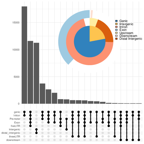
We can also visualise the annotation summary:
pdf("AnnotVis.pdf")
upsetplot(bed.annot, vennpie=TRUE)
dev.off()
Visualisation of ATAC peaks annotations.
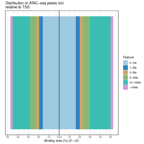
Distribution of loci with respect to TSS:
pdf("TSSdist.pdf")
plotDistToTSS(bed.annot, title="Distribution of ATAC-seq peaks loci\nrelative to TSS")
dev.off()
Summary of ATAC-seq peaks relative to TSS.
Functional Analysis
Having obtained annotations to nearest genes, we can perform functional enrichment analysis to identify predominant biological themes among these genes by incorporating knowledge provided by biological ontologies, e.g. GO (Gene Ontology, Ashburner et al. 2000) and Reactome (Croft et al. 2013).
In this tutorial we use the merged consensus peaks set. This analysis can also be performed on results of differential accessibility / occupancy.
Let’s first annotate the peaks with Reactome.
Reactome pathway enrichment of genes defined as the nearest feature to the peaks:
#finding enriched Reactome pathways using chromosome 1 and 2 genes as a background
pathway.reac <- enrichPathway(as.data.frame(annot_peaks)$geneId)

#previewing enriched Reactome pathways
head(pathway.reac)
This is the result (we skip column 8, as it is very broad - contains the gene IDs in set):
> colnames(as.data.frame(pathway.reac))
[1] "ID"          "Description" "GeneRatio"   "BgRatio"     "pvalue"
[6] "p.adjust"    "qvalue"      "geneID"      "Count"

> pathway.reac[1:10,c(1:7,9)]
                         ID
R-HSA-9012999 R-HSA-9012999
R-HSA-9013149 R-HSA-9013149
R-HSA-9013148 R-HSA-9013148
R-HSA-4420097 R-HSA-4420097
R-HSA-9006925 R-HSA-9006925
R-HSA-5683057 R-HSA-5683057
R-HSA-194138   R-HSA-194138
R-HSA-449147   R-HSA-449147
R-HSA-5663202 R-HSA-5663202
R-HSA-9013106 R-HSA-9013106
                                                                                   Description
R-HSA-9012999                                                                 RHO GTPase cycle
R-HSA-9013149                                                                RAC1 GTPase cycle
R-HSA-9013148                                                               CDC42 GTPase cycle
R-HSA-4420097                                                             VEGFA-VEGFR2 Pathway
R-HSA-9006925                                     Intracellular signaling by second messengers
R-HSA-5683057                                                   MAPK family signaling cascades
R-HSA-194138                                                                 Signaling by VEGF
R-HSA-449147                                                         Signaling by Interleukins
R-HSA-5663202 Diseases of signal transduction by growth factor receptors and second messengers
R-HSA-9013106                                                                RHOC GTPase cycle
              GeneRatio   BgRatio       pvalue     p.adjust       qvalue Count
R-HSA-9012999  424/9073 443/10856 5.713537e-16 8.678863e-13 7.415570e-13   424
R-HSA-9013149  180/9073 185/10856 1.792656e-09 1.361522e-06 1.163340e-06   180
R-HSA-9013148  155/9073 159/10856 1.512873e-08 7.660180e-06 6.545166e-06   155
R-HSA-4420097   98/9073  99/10856 3.655317e-07 1.388107e-04 1.186054e-04    98
R-HSA-9006925  287/9073 309/10856 7.154392e-07 1.882887e-04 1.608815e-04   287
R-HSA-5683057  301/9073 325/10856 8.286217e-07 1.882887e-04 1.608815e-04   301
R-HSA-194138   106/9073 108/10856 8.676899e-07 1.882887e-04 1.608815e-04   106
R-HSA-449147   421/9073 462/10856 1.150075e-06 2.183704e-04 1.865845e-04   421
R-HSA-5663202  362/9073 395/10856 1.447213e-06 2.442575e-04 2.087034e-04   362
R-HSA-9013106   74/9073  74/10856 1.631772e-06 2.478661e-04 2.117868e-04    74
We can see familar terms which can be connected to sample biology: Signaling by Interleukins, MAPK family signaling cascades.
Let’s search for enriched GO terms:
pathway.GO <- enrichGO(as.data.frame(annot_peaks)$geneId, org.Hs.eg.db, ont = "MF")
These results look in agreement with analyses using reactome:
                   ID                                Description       qvalue
GO:0004674 GO:0004674   protein serine/threonine kinase activity 1.923215e-14
GO:0030695 GO:0030695                  GTPase regulator activity 2.997318e-10
GO:0045296 GO:0045296                           cadherin binding 4.941368e-09
GO:0015631 GO:0015631                            tubulin binding 8.978474e-09
GO:0060090 GO:0060090                 molecular adaptor activity 8.978474e-09
GO:0005085 GO:0005085 guanyl-nucleotide exchange factor activity 8.979500e-09
GO:0051020 GO:0051020                             GTPase binding 2.355108e-08
GO:0003779 GO:0003779                              actin binding 6.483723e-08
GO:0031267 GO:0031267                       small GTPase binding 1.222450e-07
GO:0030674 GO:0030674     protein-macromolecule adaptor activity 1.900703e-07
GO:0042578 GO:0042578        phosphoric ester hydrolase activity 2.558341e-06
Please remember that the results of functional analysis like the one presented above can be only as good as the annotations.