Motif Analyses with monaLisa
- Date:
2025-09-25
Background
So far, we have seen how transcription factor binding sites (TFBSs) or motifs can be represented and visualized in matrix form, how the position weight matrix (PWM) can be used to scan for motif hits against a reference sequence, for example like the reference genome, and how these matrices can be retrieved from public databases like Jaspar.
Now we will make use of these functionalities and use additional tools to enrich or select for TFs are likely to be key players in experimental differences we observe between different conditions. As mentioned, the effect of TF binding can be indirectly observed via associated changes in transcription, chromatin accessibility, DNA methylation and histone modifications. Given such data types, one may for example pose the question: which TFs could be explaining the observed changes in accessibility we see? To address such questions, we will be using the Bioconductor package called monaLisa, short for motif analysis with Lisa.
Learning outcomes
Be aware of potential sequence composition biases before motif enrichment analysis.
Perfrom binned motif enrichment analysis and be able to interpret the results.
Select motifs via regression framework.
Understand the nuances and differences between both approaches.
Libraries
We start by loading the needed packages. If necessary, use
BiocManager::install() to install missing packages. Note that we
will need to work with the latest version of monaLisa if using
ggplo2>=4.0.0.
suppressPackageStartupMessages({
  library(monaLisa)
  library(BiocParallel)
  library(ggplot2)
  library(ComplexHeatmap)
  library(circlize)
  library(GenomicRanges)
  library(BSgenome.Mmusculus.UCSC.mm39)
  library(JASPAR2024)
  library(TFBSTools)
  library(SummarizedExperiment)
  library(RSQLite)
})

# ## To install the latest tool versions, and from the current bioconductor release (3.21)
# pkgs <- c("monaLisa", "BiocParallel", "ggplot2", "ComplexHeatmap", "circlize",
#           "GenomicRanges", "BSgenome.Mmusculus.UCSC.mm39", "JASPAR2024", "TFBSTools",
#           "SummarizedExperiment", "RSQLite")
# bioc <- "3.21" # with R 4.5
# #libPath <- "/path/to/custom/folder/if/desired"
# BiocManager::install(pkgs = pkgs,
#                      update = TRUE,
#                      ask = TRUE,
#                      checkBuilt = FALSE,
#                      force = FALSE,
#                      # lib = libPath,
#                      version = bioc)

# ## if you need to install a specific version of a package you can do so as follows
# remotes::install_version("ggplot2", version = "3.5.2")
The Dataset
We give a quick recap on the dataset we are dealing with and which was
used in the ATAC-seq sections of the tutorials: When CD8+ T-cells
encounter antigens they expand and differentiate into effector cells,
undergoing marked changes on the chromatin and gene expression levels.
Tsao, Kaminski et al.
investigated how these changes depend on the basic leucine zipper
ATF-like transcription factor Batf. To this end, they generated
inducible Batf conditional knock out (cKO) CD8+ T-cells derived from the
P14 T-cell receptor transgenic mouse. The Batf cKO P14 CD8+ T-cells were
transferred to recipient mice, which were then infected with the
lymphocytic choriomeningitis virus to drive the CD8+ T-cells into
differentiation to effector cells. These cells were sorted and collected
for ATAC-seq. Here we use this dataset to look at the differences in
accessibility between Batf-cKO and Wt and ask the question,
which TFs could explain these observed changes in accessibility?
We start by loading in the RDS file called
FiltPeaks.DA.TMM.annot.rds which was generated in previous
exercises. This is a GRanges object containing the annotated merged
peak regions, as well as log-fold changes in accessibility for
Batf-cKO vs Wt. We will subset the enhancer peaks which we
define as being at least 1kb away from any TSS. We will rely on the
annotations column to extract these regions. This includes the regions
called “Promoter (1-2kb)”, “Promoter (2-3kb)” and “Distal Intergenic”.
If you have run the exercises and produced the
FiltPeaks.DA.TMM.annot.rds object, you may read that file in.
Alternatively, you can download the RDS file we need from
rackham as follows. Open a terminal and type in:
<!-- # got to your working dir -->
<!-- cd /your/wdir/ -->

# make data dir
mkdir data

# download data from rackham
scp -r <username>@rackham.uppmax.uu.se:/proj/epi2025/atacseq_proc/results/DA/objects/FiltPeaks.DA.TMM.annot.rds data
Let’s read in this file.
# read in the GRanges object
gr <- readRDS("data/FiltPeaks.DA.TMM.annot.rds")
gr
GRanges object with 64900 ranges and 13 metadata columns:
        seqnames              ranges strand |             peakID        logFC
           <Rle>           <IRanges>  <Rle> |        <character>    <numeric>
      1       17   66268427-66269247      * | merged_peaks_28038     -1.61077
      2        6 122504236-122505014      * | merged_peaks_51767     -1.50849
      3        1 155076669-155077704      * |  merged_peaks_2997     -1.51788
      4        1   95195320-95196614      * |  merged_peaks_1873     -1.15764
      5        2 162944874-162945676      * | merged_peaks_36974     -1.14102
    ...      ...                 ...    ... .                ...          ...
  64896        5 108776489-108778144      * | merged_peaks_47263  4.47468e-06
  64897       12 112545059-112545410      * | merged_peaks_15084 -3.28064e-05
  64898        X 157942836-157943040      * | merged_peaks_64640 -1.50181e-05
  64899        8 124532298-124532993      * | merged_peaks_59589 -5.77357e-06
  64900        2 127180736-127181714      * | merged_peaks_35900  3.16729e-06
                FDR        gc             annotation   geneChr geneStart
          <numeric> <numeric>            <character> <integer> <integer>
      1 1.11065e-85  0.436054      Distal Intergenic        17  66261129
      2 1.08402e-82  0.480103 Intron (ENSMUST00000..         6 122499458
      3 2.05814e-77  0.500965                 3' UTR         1 155070767
      4 6.69054e-69  0.461776      Distal Intergenic         1  95183688
      5 3.50249e-68  0.503113      Distal Intergenic         2 162934819
    ...         ...       ...                    ...       ...       ...
  64896     0.99997  0.589372       Promoter (<=1kb)         5 108777636
  64897     0.99997  0.542614      Distal Intergenic        12 112555218
  64898     0.99997  0.487805      Distal Intergenic        20 157868216
  64899     0.99997  0.652299       Promoter (<=1kb)         8 124532724
  64900     0.99997  0.526047       Promoter (<=1kb)         2 127180559
          geneEnd geneStrand             geneId       transcriptId
        <integer>  <integer>        <character>        <character>
      1  66265392          1 ENSMUSG00000139744 ENSMUST00000355127
      2 122505594          1 ENSMUSG00000030116 ENSMUST00000126357
      3 155077993          1 ENSMUSG00000026470 ENSMUST00000194158
      4  95184535          2 ENSMUSG00000099592 ENSMUST00000190584
      5 162934943          1 ENSMUSG00002076785 ENSMUST00020181897
    ...       ...        ...                ...                ...
  64896 108791896          1 ENSMUSG00000013495 ENSMUST00000146207
  64897 112581391          1 ENSMUSG00000037679 ENSMUST00000101029
  64898 157929646          2 ENSMUSG00000138115 ENSMUST00000345594
  64899 124562026          1 ENSMUSG00000019478 ENSMUST00000118535
  64900 127199571          1 ENSMUSG00000050468 ENSMUST00000059839
        external_gene_name distanceToTSS
               <character>     <numeric>
      1            Gm65735          7298
      2              Mfap5          4778
      3               Stx6          5902
      4             Gm5264        -10785
      5            Gm56299         10055
    ...                ...           ...
  64896            Tmem175             0
  64897               Inf2         -9808
  64898            Gm61902        -13190
  64899              Rab4a             0
  64900               Astl           177
  -------
  seqinfo: 21 sequences from an unspecified genome; no seqlengths
# keep enhancers at least 1kb away from any TSS and not in any gene
keep <- gr$annotation %in% c("Distal Intergenic", "Promoter (1-2kb)", "Promoter (2-3kb)")
gr <- gr[keep]
table(gr$annotation)
Distal Intergenic  Promoter (1-2kb)  Promoter (2-3kb)
             9701              5633              4469
# specify chr naming convention
seqlevelsStyle(BSgenome.Mmusculus.UCSC.mm39) <- "NCBI"

# subset autosomal enhancers
keep <- seqnames(gr) %in% 1:19
gr <- gr[keep]
table(gr$annotation)
Distal Intergenic  Promoter (1-2kb)  Promoter (2-3kb)
             9392              5550              4419
# fix enhancer names
names(gr) <- paste0("e_", 1:length(gr))
head(gr)
GRanges object with 6 ranges and 13 metadata columns:
      seqnames              ranges strand |             peakID     logFC
         <Rle>           <IRanges>  <Rle> |        <character> <numeric>
  e_1       17   66268427-66269247      * | merged_peaks_28038  -1.61077
  e_2        1   95195320-95196614      * |  merged_peaks_1873  -1.15764
  e_3        2 162944874-162945676      * | merged_peaks_36974  -1.14102
  e_4       19   17241967-17242651      * | merged_peaks_31308  -1.36160
  e_5        6 122509800-122510274      * | merged_peaks_51769  -1.10413
  e_6       17   87180093-87180462      * | merged_peaks_28593  -1.80282
              FDR        gc        annotation   geneChr geneStart   geneEnd
        <numeric> <numeric>       <character> <integer> <integer> <integer>
  e_1 1.11065e-85  0.436054 Distal Intergenic        17  66261129  66265392
  e_2 6.69054e-69  0.461776 Distal Intergenic         1  95183688  95184535
  e_3 3.50249e-68  0.503113 Distal Intergenic         2 162934819 162934943
  e_4 1.86157e-52  0.436496  Promoter (1-2kb)        19  17243348  17243702
  e_5 2.66334e-43  0.475789 Distal Intergenic         6 122499458 122505594
  e_6 2.51476e-42  0.443243 Distal Intergenic        17  87147458  87148144
      geneStrand             geneId       transcriptId external_gene_name
       <integer>        <character>        <character>        <character>
  e_1          1 ENSMUSG00000139744 ENSMUST00000355127            Gm65735
  e_2          2 ENSMUSG00000099592 ENSMUST00000190584             Gm5264
  e_3          1 ENSMUSG00002076785 ENSMUST00020181897            Gm56299
  e_4          2 ENSMUSG00000117946 ENSMUST00000237419            Gm50280
  e_5          1 ENSMUSG00000030116 ENSMUST00000126357              Mfap5
  e_6          1 ENSMUSG00000099798 ENSMUST00000189953            Gm29168
      distanceToTSS
          <numeric>
  e_1          7298
  e_2        -10785
  e_3         10055
  e_4          1051
  e_5         10342
  e_6         32635
  -------
  seqinfo: 21 sequences from an unspecified genome; no seqlengths
Let us have a look at the enhancers we have and check if there is a relationship between logFC and GC content. We have already done quality checks like this in previous sections of the tutorial. Are there any sequence biases associated with the log-fold changes in accessibility?
# logFC vs GC content
par(mfrow=c(1,2))
plot(gr$gc, gr$logFC, pch = ".")
abline(h = 0, col = "red", lty = 5)
smoothScatter(gr$gc, gr$logFC)
abline(h = 0, col = "red", lty = 5)
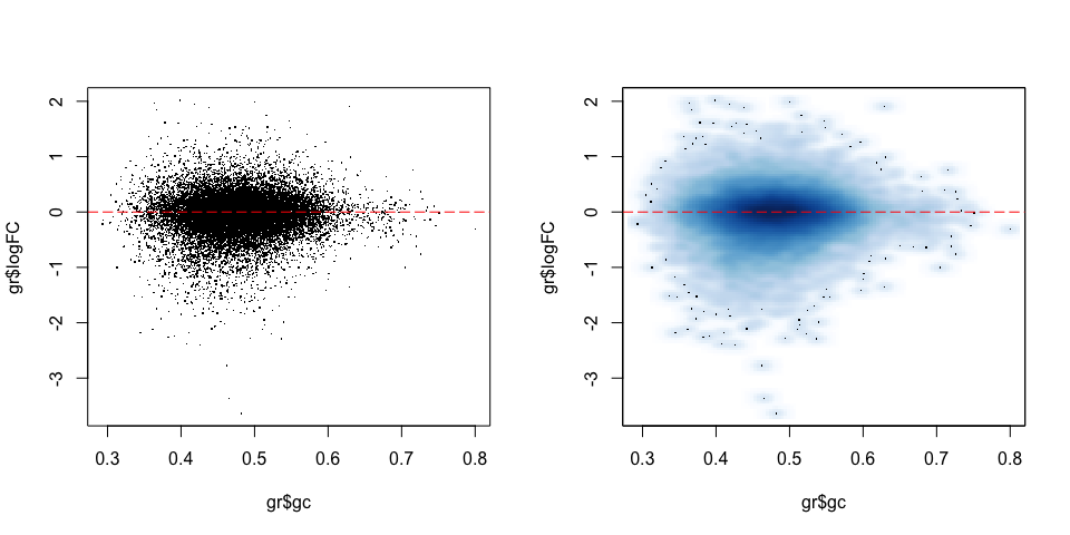
We see no dependence of the logFC in accessibility on the GC content. This is also what we have seen previously.
As mentioned, we posed the question: which motifs could explain the
changes in accessibility we see between Batf-cKO and Wt. To
predict and select potential motifs, we will use the monaLisa
package, which offers two main approaches:
Binned enrichment approach: the enhancer sequences are binned by their logFC, and motif enrichment is calculated in each bin vs the rest. This is done independently for each motif. Internally, this approach utilizes the sequence composition corrections between foreground and background sequences which Homer does.
Regression approach: here motifs compete against each other for selection and those that are more likely to explain the logFCs are selected.
Both approaches are valid ways to answer the question we posed, but do so from a different angle. More details on both approaches will be described below as we explore and apply them to our dataset.
Binned motif enrichment analysis
For this approach we are closely following the main
vignette
from monaLisa. Briefly, we will take the logFC vector across
enhancer regions, draw a histogram of the logFCs, bin the histogram,
test for motif enrichment per bin for each TF and finally visualize the
results.
Bin by log-fold changes in accessibility
Before proceeding with the motif enrichment analysis, we want to make sure that the regions we are using have similar sizes, to avoid any length biases in the comparisons between the different bins. We will resize the regions to a fixed size around the midpoint of each region, corresponding to the median region size.
# region size distribution
summary(width(gr))
 Min. 1st Qu.  Median    Mean 3rd Qu.    Max.
112.0   325.0   445.0   511.8   618.0  8618.0
# resize the regions and trim out-of bounds ranges
gr <- trim(resize(gr, width = median(width(gr)), fix = "center"))
summary(width(gr))
Min. 1st Qu.  Median    Mean 3rd Qu.    Max.
 445     445     445     445     445     445
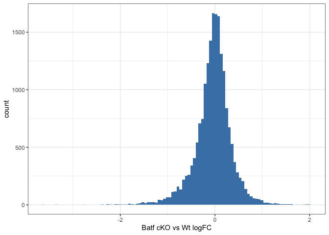
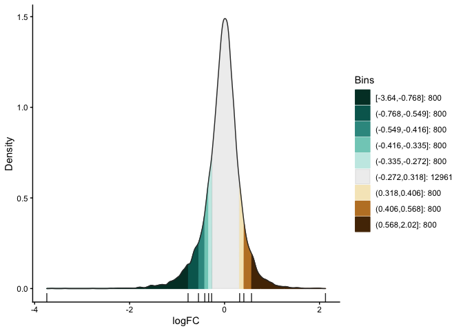
Let us examine the histogram depicting the logFCs across the enhancers and create bins. In order to have robust calculations in enrichment, it is recommended to have at least a couple of hundred sequences per bin. Here, we will have 800 regions or sequences per bin, and additionally set a min absolute logFC above which to bin.
# plot logFC histogram
ggplot(data = data.frame(logFC = gr$logFC)) +
  geom_histogram(aes(x = logFC), bins = 100, fill = "steelblue") +
  xlab("Batf cKO vs Wt logFC") +
  theme_bw()
# bin the histogram
bins <- bin(x = gr$logFC, binmode = "equalN", nElement = 800,
            minAbsX = 0.3)

table(bins)
bins
 [-3.64,-0.768] (-0.768,-0.549] (-0.549,-0.416] (-0.416,-0.335] (-0.335,-0.272]
            800             800             800             800             800
 (-0.272,0.318]   (0.318,0.406]   (0.406,0.568]    (0.568,2.02]
          12961             800             800             800
# plot binned histogram
plotBinDensity(x = gr$logFC, b = bins) +
  xlab("logFC")
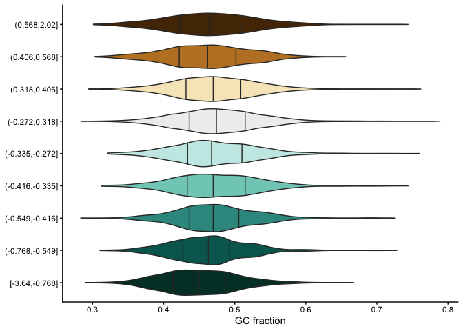
Before proceeding with the enrichment analysis, let’s check if there is
any sequence bias associated with the bins. monaLisa offers some
plotting functions for this purpose.
# extract DNA sequences of the enhancers
seqs <- getSeq(BSgenome.Mmusculus.UCSC.mm39, gr)

# by GC fraction
plotBinDiagnostics(seqs = seqs, bins = bins, aspect = "GCfrac")
# by dinucleotide frequency
plotBinDiagnostics(seqs = seqs, bins = bins, aspect = "dinucfreq")
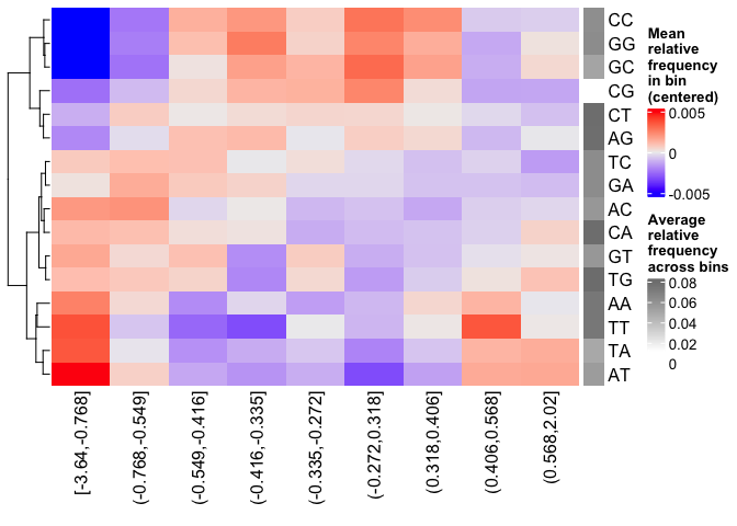
We note a small tendency for the bin with the most negative logFC values to have lower GC content. This is also reflected in the heatmap with the dinucleotide frequencies, with that (first) bin being slightly more AT-rich. We will keep this in mind when we examine the enriched motifs. We will want to see if mostly GC-poor motifs are enriched in this bin. That could indicate that the built-in sequence composition corrections were not enough. For now we just make note of it.
Get PWMs from Jaspar
We load the PWMs of vertebrate TFs from Jaspar.
# extract PWMs of vertebrate TFs from JASPAR2024
JASPAR2024 <- JASPAR2024()
JASPARConnect <- RSQLite::dbConnect(RSQLite::SQLite(), db(JASPAR2024))
pwms <- getMatrixSet(JASPARConnect,
                     opts = list(tax_group = "vertebrates",
                                 collection="CORE",
                                 matrixtype = "PWM"))

# disconnect Db
RSQLite::dbDisconnect(JASPARConnect)
Run binned enrichment
We can now run the motif enrichment analysis. We will do the enrichment
per bin vs all other bins, which is the default option in
calcBinnedMotifEnrR. To learn more about the other available
options, which can be controlled via the background parameter, see
the help page of the function.
The p-value for the enrichment test is calculated using Fisher’s exact test. We illustrate the contingency table used for this test below. Given a specific bin, for each motif, we end up with a table of weighted counts as shown below. They are weighted to correct for sequence composition differences between the foreground and background sets, where foreground reflects the sequences belonging to the bin being tested, and background sequences from all other bins.
with TF hit |
with no TF hit |
|
|---|---|---|
foreground |
a |
b |
background |
c |
d |
# motif enrichment using 4 cores
se <- calcBinnedMotifEnrR(seqs = seqs,
                          bins = bins,
                          pwmL = pwms,
                          background = "otherBins",
                          BPPARAM = MulticoreParam(4))
se
class: SummarizedExperiment
dim: 879 9
metadata(5): bins bins.binmode bins.breaks bins.bin0 param
assays(7): negLog10P negLog10Padj ... sumForegroundWgtWithHits
  sumBackgroundWgtWithHits
rownames(879): MA0004.1 MA0069.1 ... MA1602.2 MA1722.2
rowData names(5): motif.id motif.name motif.pfm motif.pwm
  motif.percentGC
colnames(9): [-3.64,-0.768] (-0.768,-0.549] ... (0.406,0.568]
  (0.568,2.02]
colData names(6): bin.names bin.lower ... totalWgtForeground
  totalWgtBackground
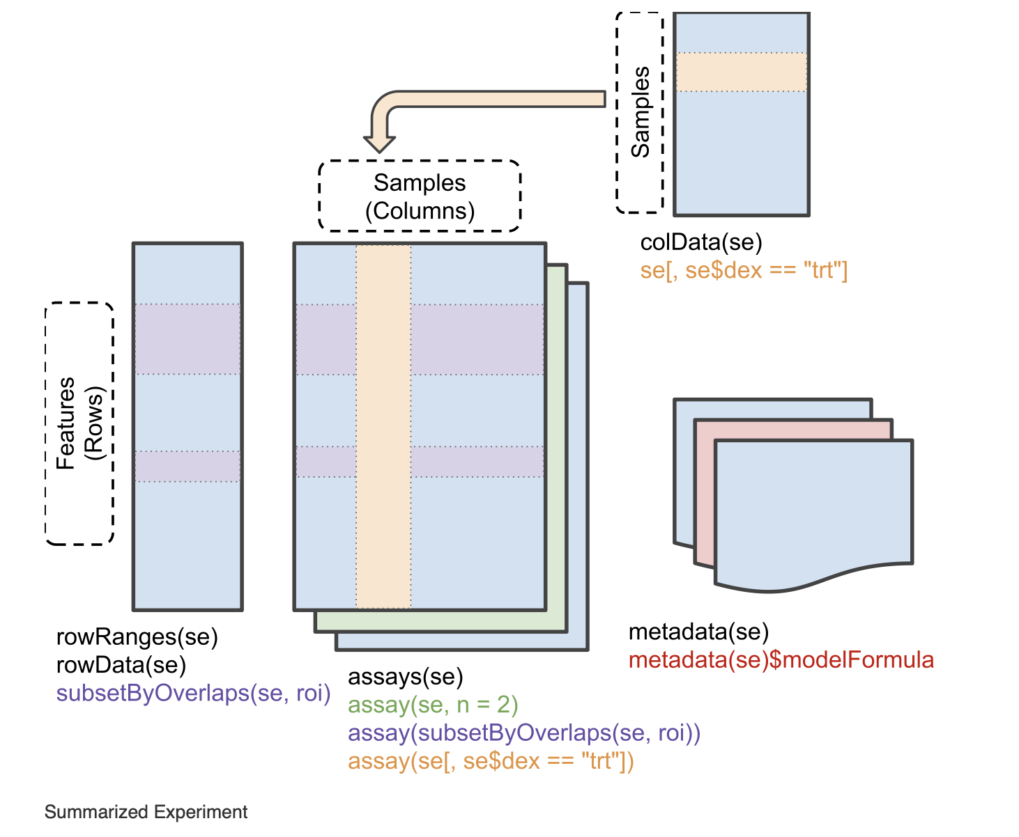
The resulting object is a SummarizedExperiment object. Briefly,
these classes are a convenient way to store matrices of the same
dimensions as well as any row and column metadata. In our case, the rows
correspond to the motifs and the columns to the bins. The figure below
illustrates what this class of objects looks like and more details can
be found on
Bioconductor.
# assays (matrices)
assays(se)
List of length 7
names(7): negLog10P negLog10Padj ... sumBackgroundWgtWithHits
head(assays(se)$log2enr)
         [-3.64,-0.768] (-0.768,-0.549] (-0.549,-0.416] (-0.416,-0.335]
MA0004.1     0.05597966      0.04640559    -0.189753535     -0.06415103
MA0069.1     0.17975718      0.25349055     0.150531770      0.13207467
MA0071.1     0.16204117      0.07953121    -0.038933264      0.05030480
MA0074.1    -0.28030942      0.04941143     0.016441742      0.09012599
MA0101.1     0.04348448      0.15824544    -0.004039081      0.04565927
MA0107.1     0.11901851      0.21733994    -0.124788897      0.10166630
         (-0.335,-0.272] (-0.272,0.318] (0.318,0.406] (0.406,0.568]
MA0004.1     -0.32381212     0.07752202    0.24423267    0.11737879
MA0069.1      0.10083004    -0.11308572   -0.02621159   -0.19109729
MA0071.1     -0.03616484    -0.02764498   -0.01907538   -0.03344962
MA0074.1     -0.32978473     0.23169199   -0.17188287   -0.37803402
MA0101.1     -0.28496525    -0.05683605    0.03327832    0.05179975
MA0107.1     -0.10959571    -0.08295046   -0.19209122    0.17039864
         (0.568,2.02]
MA0004.1  -0.15042189
MA0069.1  -0.01945742
MA0071.1   0.01519093
MA0074.1  -0.09446126
MA0101.1   0.25093533
MA0107.1   0.17052358
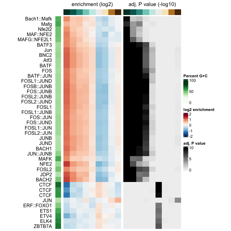
Let’s visualize the results of the enrichment analysis. We can use the
plot function provided by monaLisa to do this.
# select strongly enriched motifs
sel <- apply(assay(se, "negLog10Padj"), 1,
             function(x) max(abs(x), 0, na.rm = TRUE)) > 4.0
sum(sel)
[1] 41
seSel <- se[sel, ]

# plot
plotMotifHeatmaps(x = seSel, which.plots = c("log2enr", "negLog10Padj"),
                  width = 2.0, cluster = TRUE, maxEnr = 2, maxSig = 10,
                  show_motif_GC = TRUE)
# plot with motif sequence logos
SimMatSel <- motifSimilarity(rowData(seSel)$motif.pfm)
range(SimMatSel)
[1] 0.1332093 1.0000000
# create hclust object, similarity defined by 1 - Pearson correlation
hcl <- hclust(as.dist(1 - SimMatSel), method = "average")
plotMotifHeatmaps(x = seSel, which.plots = c("log2enr", "negLog10Padj"),
                  width = 1.8, cluster = hcl, maxEnr = 2, maxSig = 10,
                  show_dendrogram = TRUE, show_seqlogo = TRUE,
                  width.seqlogo = 1.2)
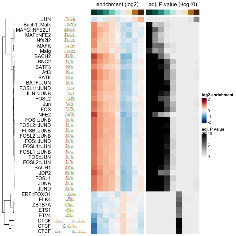
The Fos/Jun motif is particularly enriched in bins corresponding to negative logFC values, so regions which lost accessibility in the BatfKO. Coming back to our earlier note of a tendency to have GC-poor sequences in the first bin with the most negative logFCs, we don’t see purely AT-rich motifs enriched in this bin, hinting that the internal sequence bias corrections were good enough. Furthermore, The rest of the bins with negative logFCs also show enrichments of the Fos/Jun motif. Seeing a gradient of enrichment the more extreme the logFC values are adds another layer of confidence in the enrichment results.
Binned k-mer enrichment analysis
Sometimes one may want to perform the binned enrichment analysis in a more unbiased way, without using known motifs from a database. We perform this on our dataset and look at which kmers are enriched. We will set the kmer size to 6 base pairs.
# binned kmer enrichment
seKmer <-  calcBinnedKmerEnr(seqs = seqs, bins = bins, kmerLen = 6,
                          includeRevComp = TRUE, BPPARAM = MulticoreParam(4))

# enriched kmers
selKmer <- apply(assay(seKmer, "negLog10Padj"), 1,
               function(x) max(abs(x), 0, na.rm = TRUE)) > 4
sum(selKmer)
[1] 14
seKmerSel <- seKmer[selKmer, ]

# calculate similarity between enriched kmers and enriched motifs
pfmSel <- rowData(seSel)$motif.pfm
sims <- motifKmerSimilarity(x = pfmSel,
                            kmers = rownames(seKmerSel),
                            includeRevComp = TRUE)
dim(sims)
[1] 41 14
# plot kmers and motif similarity
maxwidth <- max(sapply(TFBSTools::Matrix(pfmSel), ncol))
seqlogoGrobs <- lapply(pfmSel, seqLogoGrob, xmax = maxwidth)
hmSeqlogo <- rowAnnotation(logo = annoSeqlogo(seqlogoGrobs, which = "row"),
                           annotation_width = unit(1.5, "inch"),
                           show_annotation_name = FALSE
)

Heatmap(sims,
        show_row_names = TRUE, row_names_gp = gpar(fontsize = 8),
        show_column_names = TRUE, column_names_gp = gpar(fontsize = 8),
        name = "Similarity", column_title = "Selected TFs and enriched k-mers",
        col = colorRamp2(c(0, 1), c("white", "red")),
        right_annotation = hmSeqlogo)
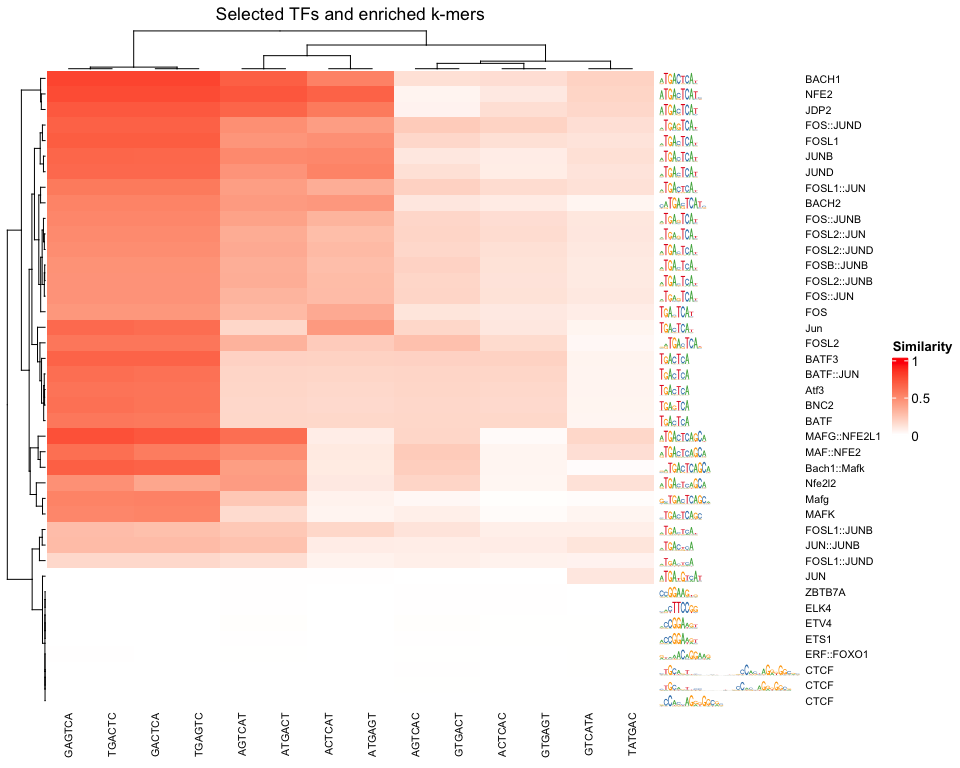
We can appreciate the enriched k-mers corresponding to the enriched motifs from earlier.
Regression-based analysis
Another method to find relevant motifs is via a regression-based
approach. As opposed to the binned approach, where each motif is tested
independently for enrichment, the regression framework allows motifs to
compete against each other for selection. Following our example, the aim
is to select those which are more likely to explain the observed changes
in accessibilty we see across the enhancers. In monaLisa, stability
selection with randomized lasso is the implemented regression method of
choice. For more details about the method, see the details section in
the randLassoStabSel function, as well as the publication from
Meinshausen and
Bühlmann. Briefly,
with lasso stability selection, the lasso regression is performed
multiple times on subsets of the response vector and predictor matrix,
and each predictor (TF) end up with a selection probability which is
simply the number of times it was selected divided by the total number
of times a regression was done. With the randomized lasso, a weakness
parameter is additionally used to vary the lasso penalty term λ to a
randomly chosen value between [λ, λ/weakness] for each predictor. This
type of regularization has advantages in cases where the number of
predictors exceeds the number of observations, in selecting variables
consistently, demonstrating better error control and not depending
strongly on the penalization parameter (Meinshausen and Bühlmann 2010).
First, we will create the predictor matrix in our regression framework. This will consist of the predicted TF binding sites (TFBSs) across the enhancers. We use the PWMs from Jaspar to scan for motif hits across the enhancers, using a minimum score of 10 for a match.
# scan for motif hits across enhancer sequences
#   (this step takes a few seconds)
hits <- findMotifHits(query = pwms, subject = seqs, min.score = 10.0,
                      BPPARAM = BiocParallel::MulticoreParam(4))
head(hits)
GRanges object with 6 ranges and 4 metadata columns:
      seqnames    ranges strand |     matchedSeq    pwmid pwmname     score
         <Rle> <IRanges>  <Rle> | <DNAStringSet>    <Rle>   <Rle> <numeric>
  [1]      e_1       1-8      + |       AAGTGTGA MA0801.1     MGA   11.3951
  [2]      e_1       1-8      + |       AAGTGTGA MA0803.1   TBX15   10.8442
  [3]      e_1       1-8      + |       AAGTGTGA MA0805.1    TBX1   12.1899
  [4]      e_1       1-8      + |       AAGTGTGA MA0806.1    TBX4   11.1102
  [5]      e_1       1-8      + |       AAGTGTGA MA0807.1    TBX5   10.0778
  [6]      e_1       1-9      + |      AAGTGTGAG MA0800.2   EOMES   10.1016
  -------
  seqinfo: 19361 sequences from an unspecified genome
# add columns reflecting motif ID and name (for ease of interpretability later)
hits$pwmIdName <- paste0(hits$pwmid, "_", hits$pwmname)

# create TFBS matrix (unique motif IDs are shown as columns rather than the names)
TFBSmatrix <- unclass(table(factor(seqnames(hits), levels = seqlevels(hits)),
                            factor(hits$pwmIdName, levels = unique(hits$pwmIdName))))
TFBSmatrix[1:6, 1:6]
    MA0801.1_MGA MA0803.1_TBX15 MA0805.1_TBX1 MA0806.1_TBX4 MA0807.1_TBX5
e_1            7              7             7             7             7
e_2            0              0             0             0             0
e_3            1              1             1             1             1
e_4            0              0             0             0             0
e_5            1              1             1             1             1
e_6            0              0             0             1             0

    MA0800.2_EOMES
e_1             10
e_2              0
e_3              1
e_4              0
e_5              1
e_6              0
# remove TF motifs with 0 binding sites (if any) in all regions
zero_TF <- colSums(TFBSmatrix) == 0
sum(zero_TF)
[1] 0
TFBSmatrix <- TFBSmatrix[, !zero_TF]
We add the fraction of G+C and CpG observed/expected ratio as predictors to the matrix, to ensure that selected TF motifs are not just detecting a simple trend in GC or CpG composition.
# calculate G+C and CpG obs/expected
fMono <- oligonucleotideFrequency(seqs, width = 1L, as.prob = TRUE)
fDi <- oligonucleotideFrequency(seqs, width = 2L, as.prob = TRUE)
fracGC <- fMono[, "G"] + fMono[, "C"]
oeCpG <- (fDi[, "CG"] + 0.01) / (fMono[, "G"] * fMono[, "C"] + 0.01)

# add GC and oeCpG to predictor matrix
TFBSmatrix <- cbind(fracGC, oeCpG, TFBSmatrix)
TFBSmatrix[1:6, 1:6]
       fracGC     oeCpG MA0801.1_MGA MA0803.1_TBX15 MA0805.1_TBX1 MA0806.1_TBX4
e_1 0.4269663 0.2625459            7              7             7             7
e_2 0.4876404 0.4251465            0              0             0             0
e_3 0.4674157 0.4697612            1              1             1             1
e_4 0.4471910 0.4351891            0              0             0             0
e_5 0.4786517 0.3186635            1              1             1             1
e_6 0.4539326 0.3939226            0              0             0             1
Next we run stability selection with randomized lasso. Since this is a stochastic process, we will need to set the seed to reproduce our results.
# run randomized lasso stability selection
set.seed(123)
se <- randLassoStabSel(x = TFBSmatrix, y = gr$logFC, cutoff = 0.8)
se
class: SummarizedExperiment
dim: 19361 856
metadata(12): stabsel.params.cutoff stabsel.params.selected ...
  stabsel.params.call randStabsel.params.weakness
assays(1): x
rownames(19361): e_1 e_2 ... e_19360 e_19361
rowData names(1): y
colnames(856): fracGC oeCpG ... MA2100.1_ZSCAN16 MA0735.2_GLIS1
colData names(30): selProb selected ... regStep26 regStep27
# selected TFs
sel <- colnames(se)[se$selected]
sel
[1] "MA1142.2_FOSL1::JUND" "MA0835.3_BATF3"       "MA0002.3_Runx1"
[4] "MA0791.2_POU4F3"      "MA0645.2_ETV6"
As mentioned, motifs are competing against each other for selection here. A known challenge with regression methods is colinearity between the predictors. This is worth keeping in mind for very highly correlated TFBSs. If we have two TFs with highly similar motifs explaining the logFC, only one of them may end up being selected. It is also worth remembering to focus on interpreting the motifs rather than the particular TF name.
Let’s have a look at the stability paths of the motifs. These paths show the selection probability as a function of the regularization step. The strength of the regularization decreases from left to right and the stronger the regularization, the less motifs are selected. The motifs above the minimum selection probability at the last step are the final selected ones. These paths can give an indication of how strongly a particular motif can explain the logFC in accessibility, by being selected fairly early and then consistently along the regulalrization steps. It can also show how well the selected motifs separate from the non-selected ones and how strong the signal is.
plotStabilityPaths(se, labelPaths = TRUE)
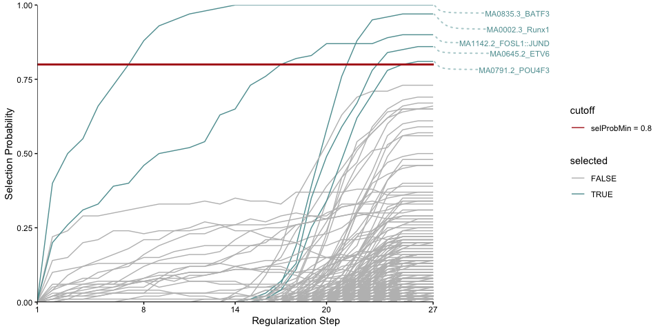
Based on these, BATF3 is the first motif to be selected which indicates that this motif quite strongly explains the logFC compared to the rest. This may be expected since this TF was knocked out.
Let’s look at where the GC and CpG content predictors fall on these paths.
plotStabilityPaths(se, labelPaths = TRUE, labelNudgeX = 3,
                   labels = c("fracGC", "oeCpG"))
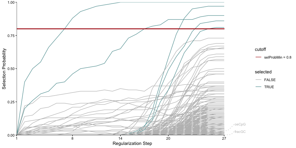
They have very low selection probabilities and were not contributing to explaining the logFC in accessibility. What if we want to get a sense of the direction in which the selected motifs explain accessibility changes: towards positive logFC values indicating more accessibility in KO, or toward negative logFC values indicating more accessibility in the Wt? To reflect that, we can plot the selection probabilities multiplied by the sign of the correlation to the logFC vector.
plotSelectionProb(se, directional = TRUE, ylimext = 1)
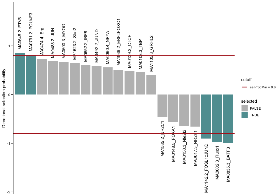
BATF3, Runx1 and FOSL1::JUND explain negative changes in accessibility, so enhancers which were more accessible in Wt and lost that accessibility in the Batf-KO. The motifs for BATF3 and FOSL1::JUND were also enriched in the binned approach, in bins with lower logFC values. Interestingly Runx1 only shows up here. Let’s have a look at the motif seqlogo to see if that motif came up in the enrichment approach under another TF name.
# get PFM
JASPAR2024 <- JASPAR2024()
JASPARConnect <- RSQLite::dbConnect(RSQLite::SQLite(), db(JASPAR2024))
pfm <- getMatrixByID(x = JASPARConnect, ID = "MA0002.3")
RSQLite::dbDisconnect(JASPARConnect)
name(pfm)
[1] "Runx1"
# plot seqlogo
seqLogo(x = toICM(pfm))

We did not see this motif in the binned approach. Perhaps this could only be selected in context with the rest of the motifs. We can also have a closer look at some of the enhancers which have predicted binding sites for a motif of interest, ordering by absolute logFC in accessibility as a means of ranking the most important ones. Let’s look at such top enhancers for the Runx1 motif.
# TF on interest
TF <- sel[3]
TF
[1] "MA0002.3_Runx1"
# identify enhancerswhich contain perdicted TFBSs
i <- which(assay(se, "x")[, TF] > 0)

# order by absolute logFC
o <- order(abs(gr$logFC[i]), decreasing = TRUE)
gr[i][o]
GRanges object with 7865 ranges and 13 metadata columns:
          seqnames              ranges strand |             peakID        logFC
             <Rle>           <IRanges>  <Rle> |        <character>    <numeric>
    e_946       17   32327657-32328101      * | merged_peaks_26931     -3.36110
    e_586        3   21776693-21777137      * | merged_peaks_38008     -2.77391
    e_940       10   76572614-76573058      * |  merged_peaks_6105     -2.28866
    e_104        8   95554605-95555049      * | merged_peaks_58633     -2.20077
    e_165        1   52458595-52459039      * |   merged_peaks_710     -2.11577
      ...      ...                 ...    ... .                ...          ...
  e_19350       15   97396226-97396670      * | merged_peaks_23110 -1.85648e-04
  e_19354        5 148713152-148713596      * | merged_peaks_49032  1.61644e-04
  e_19345        1 194914907-194915351      * |  merged_peaks_4361 -1.30662e-04
  e_19357        1   66934978-66935422      * |  merged_peaks_1135 -4.34532e-05
  e_19359       11   46321910-46322354      * |  merged_peaks_8973  4.34149e-05
                  FDR        gc        annotation   geneChr geneStart   geneEnd
            <numeric> <numeric>       <character> <integer> <integer> <integer>
    e_946 1.10436e-02  0.464912  Promoter (1-2kb)        17  32297771  32326324
    e_586 7.03546e-04  0.462500 Distal Intergenic         3  21765445  21766624
    e_940 1.06377e-02  0.536680 Distal Intergenic        10  76562417  76566107
    e_104 2.54669e-14  0.522727  Promoter (1-2kb)         8  95549649  95553342
    e_165 4.66155e-10  0.511111 Distal Intergenic         1  52466578  52469655
      ...         ...       ...               ...       ...       ...       ...
  e_19350    0.999918  0.516393 Distal Intergenic        15  97366414  97367594
  e_19354    0.999918  0.505714  Promoter (1-2kb)         5 148714721 148715615
  e_19345    0.999906  0.444238 Distal Intergenic         1 194910586 194910706
  e_19357    0.999918  0.424396  Promoter (1-2kb)         1  66935758  66936885
  e_19359    0.999918  0.473822 Distal Intergenic        11  46327752  46331685
          geneStrand             geneId       transcriptId external_gene_name
           <integer>        <character>        <character>        <character>
    e_946          2 ENSMUSG00000121449 ENSMUST00000183934            Pdxk-ps
    e_586          1 ENSMUSG00000105440 ENSMUST00000365735            Gm31693
    e_940          2 ENSMUSG00000112291 ENSMUST00000218963            Gm48276
    e_104          2 ENSMUSG00000031781 ENSMUST00000162357            Ciapin1
    e_165          1 ENSMUSG00000122096 ENSMUST00000250730            Gm69377
      ...        ...                ...                ...                ...
  e_19350          2 ENSMUSG00000143807 ENSMUST00000379400            Gm63280
  e_19354          1 ENSMUSG00000085740 ENSMUST00000335092      4930505K14Rik
  e_19345          1 ENSMUSG00002076810 ENSMUST00020183637            Gm56030
  e_19357          2 ENSMUSG00000124891 ENSMUST00000266817            Gm69843
  e_19359          1 ENSMUSG00000020397 ENSMUST00000152119               Med7
          distanceToTSS
              <numeric>
    e_946         -1385
    e_586         11271
    e_940         -6600
    e_104         -1244
    e_165         -7671
      ...           ...
  e_19350        -28733
  e_19354         -1172
  e_19345          4275
  e_19357          1292
  e_19359         -5429
  -------
  seqinfo: 21 sequences from an unspecified genome; no seqlengths
Additional resources
This tutorial has closely followed the vignettes provided in the
monaLisa package. They are referenced below, as well additional
reading material.
monaLisa’s binned motif enrichment vignette: https://bioconductor.org/packages/release/bioc/vignettes/monaLisa/inst/doc/monaLisa.htmlmonaLisa’s regression vignette: https://bioconductor.org/packages/release/bioc/vignettes/monaLisa/inst/doc/selecting_motifs_with_randLassoStabSel.htmlRecent publications which have benchmarked several tools looking at TF selection or enrichment:
Gerbaldo, F. E., Sonder, E., Fischer, V., Frei, S., Wang, J., Gapp, K., Robinson, M. D., & Germain, P.-L. (2024). On the identification of differentially-active transcription factors from ATAC-seq data. PLOS Computational Biology, 20(10), e1011971. https://doi.org/10.1371/journal.pcbi.1011971
Santana, L. S., Reyes, A., Hoersch, S., Ferrero, E., Kolter, C., Gaulis, S., & Steinhauser, S. (2024). Benchmarking tools for transcription factor prioritization. Computational and Structural Biotechnology Journal, 23, Article 1274-1287. https://doi.org/10.1016/j.csbj.2024.03.016
Stability selection paper: Meinshausen, N., & Bühlmann, P. (2010). Stability selection. Journal of the Royal Statistical Society: Series B (Statistical Methodology), 72(4), 417–473. https://doi.org/10.1111/j.1467-9868.2010.00740.x
Improved error bounds on stability selection: Shah, R. D., & Samworth, R. J. (2013). Variable selection with error control: Another look at stability selection. Journal of the Royal Statistical Society: Series B (Statistical Methodology), 75(1), 55–80. https://doi.org/10.1111/j.1467-9868.2011.01034.x
Session
date()
[1] "Thu Sep 25 13:58:54 2025"
sessionInfo()
R version 4.5.1 (2025-06-13)
Platform: aarch64-apple-darwin20
Running under: macOS Sequoia 15.6.1

Matrix products: default
BLAS:   /Library/Frameworks/R.framework/Versions/4.5-arm64/Resources/lib/libRblas.0.dylib
LAPACK: /Library/Frameworks/R.framework/Versions/4.5-arm64/Resources/lib/libRlapack.dylib;  LAPACK version 3.12.1

locale:
[1] en_US.UTF-8/en_US.UTF-8/en_US.UTF-8/C/en_US.UTF-8/en_US.UTF-8

time zone: Europe/Stockholm
tzcode source: internal

attached base packages:
[1] stats4    grid      stats     graphics  grDevices utils     datasets
[8] methods   base

other attached packages:
 [1] RSQLite_2.4.3                      SummarizedExperiment_1.38.1
 [3] Biobase_2.68.0                     MatrixGenerics_1.20.0
 [5] matrixStats_1.5.0                  TFBSTools_1.46.0
 [7] JASPAR2024_0.99.7                  BiocFileCache_2.16.0
 [9] dbplyr_2.5.0                       BSgenome.Mmusculus.UCSC.mm39_1.4.3
[11] BSgenome_1.76.0                    rtracklayer_1.68.0
[13] BiocIO_1.18.0                      Biostrings_2.76.0
[15] XVector_0.48.0                     GenomicRanges_1.60.0
[17] GenomeInfoDb_1.44.0                IRanges_2.42.0
[19] S4Vectors_0.46.0                   BiocGenerics_0.54.0
[21] generics_0.1.4                     circlize_0.4.16
[23] ComplexHeatmap_2.24.1              ggplot2_4.0.0
[25] BiocParallel_1.42.2                monaLisa_1.14.1

loaded via a namespace (and not attached):
 [1] DBI_1.2.3                   bitops_1.0-9
 [3] stabs_0.6-4                 rlang_1.1.6
 [5] magrittr_2.0.3              clue_0.3-66
 [7] GetoptLong_1.0.5            compiler_4.5.1
 [9] png_0.1-8                   vctrs_0.6.5
[11] pwalign_1.4.0               pkgconfig_2.0.3
[13] shape_1.4.6.1               crayon_1.5.3
[15] fastmap_1.2.0               labeling_0.4.3
[17] caTools_1.18.3              Rsamtools_2.24.1
[19] rmarkdown_2.29              UCSC.utils_1.4.0
[21] DirichletMultinomial_1.50.0 purrr_1.0.4
[23] bit_4.6.0                   xfun_0.52
[25] glmnet_4.1-9                cachem_1.1.0
[27] jsonlite_2.0.0              blob_1.2.4
[29] DelayedArray_0.34.1         parallel_4.5.1
[31] cluster_2.1.8.1             R6_2.6.1
[33] RColorBrewer_1.1-3          Rcpp_1.1.0
[35] iterators_1.0.14            knitr_1.50
[37] Matrix_1.7-4                splines_4.5.1
[39] tidyselect_1.2.1            abind_1.4-8
[41] yaml_2.3.10                 doParallel_1.0.17
[43] codetools_0.2-20            curl_6.4.0
[45] lattice_0.22-7              tibble_3.3.0
[47] withr_3.0.2                 S7_0.2.0
[49] evaluate_1.0.4              survival_3.8-3
[51] pillar_1.11.0               filelock_1.0.3
[53] KernSmooth_2.23-26          foreach_1.5.2
[55] RCurl_1.98-1.17             scales_1.4.0
[57] gtools_3.9.5                glue_1.8.0
[59] seqLogo_1.74.0              tools_4.5.1
[61] TFMPvalue_0.0.9             GenomicAlignments_1.44.0
[63] XML_3.99-0.18               Cairo_1.6-2
[65] tidyr_1.3.1                 colorspace_2.1-1
[67] GenomeInfoDbData_1.2.14     restfulr_0.0.16
[69] cli_3.6.5                   S4Arrays_1.8.1
[71] dplyr_1.1.4                 gtable_0.3.6
[73] digest_0.6.37               ggrepel_0.9.6
[75] SparseArray_1.8.0           rjson_0.2.23
[77] farver_2.1.2                memoise_2.0.1
[79] htmltools_0.5.8.1           lifecycle_1.0.4
[81] httr_1.4.7                  GlobalOptions_0.1.2
[83] bit64_4.6.0-1