MINUTE-ChIP
Background
Quantitative ChIP-seq methods allow us to compare the effect of DNA-protein interactions across samples. In our lab we developed MINUTE-ChIP, a multiplexed quantitative ChIP-seq method.
To process the raw data produced with this method, we developed minute. minute takes multiplexed MINUTE-ChIP FASTQ files and outputs a set of normalized, scaled bigWig files that can be directly compared across conditions.
If you want to know more about the minute pipeline workflow , you can check out our biorXiv preprint [1].
This tutorial has two parts:
Primary analysis: Run a minute workflow on a small set of FASTQ files.
Downstream analysis: Look at the resulting bigWig files using usual bioinformatics tools.
We are going to analyse H3K27m3 data from human ESCs, where we have shown that Naive cells’ H3K27m3 landscape looks very different when compared to Primed cells in a quantitative manner. This dataset comes from our publication [2].
In order to make this tutorial last a reasonable time, the primary analysis part is independent from the second part, as it runs only on a subset of the data you can see in the second part. During the primary analysis you will see H3K27m3 data output for replicate 1 of our experiments. In the downstream analysis you can look at the genome-wide values and at relevant loci, such as bivalent genes.
What you will learn:
Apply the
minutedata-processing pipeline to a set of MINUTE-ChIP fastq files.Visualize differences between unscaled and scaled bigWig files, using standard tools like IGV, deepTools, R.
Understand how quantitative ChIP results are different from traditional ChIP, using as example H3K27m3 data on human ESCs.
Primary analysis
minute runs on Snakemake, a workflow management system that is based on python and inspired on Makefile rules. You will learn more about workflow management on the Nextflow and nf-core tutorials, but let this first part of the tutorial serve as an example of how to run a different workflow, and give you an idea of how a MINUTE-ChIP analysis goes end-to-end.
Conda environment
To make sure you have all the necessary tools to run minute, you can use a conda environment. There is a pre-made version of this environment on:
/sw/courses/epigenomics/quantitative_chip_simon/condaenv/minute so you can just:
module load bioinfo-tools
module load conda

conda activate /sw/courses/epigenomics/quantitative_chip_simon/condaenv/minute
Optional: If you want to make a fresh install, you can make a new conda environment and install minute in it. However this could take a little while:
module load bioinfo-tools
module load conda

conda create -n minute minute
Files
We are going to look at Naïve vs Primed human ES cells, and as control we have EZH2-inhibitor treatment, which removes H3K27m3 from the cells, creating a baseline for technical background.
There are 3 replicates for each condition. In the first part of the tutorial you will run replicate 1, and results for all replicates are precalculated and available in the second part.
# Create your primary analysis directory
mkdir -p my_primary/fastq
cd my_primary/fastq

# Create symlinks to our fastq files
for i in /sw/courses/epigenomics/quantitative_chip_simon/minute_tutorial/primary/*.fastq.gz; do ln -s ${i}; done
cd ..
cp /sw/courses/epigenomics/quantitative_chip_simon/minute_tutorial/primary/*.tsv .
cp /sw/courses/epigenomics/quantitative_chip_simon/minute_tutorial/primary/*.yaml .
Now, this is how your directory structure should look like:
fastq/- Contains all the fastq.gz files in the table below.libraries.tsv- Specifies how the samples are demultiplexed.groups.tsv- Specifies how the samples are scaled.minute.yaml- Some extra config values. Where the references are, how long is the UMI.
Configuration
minute needs these three configuration files to run:
minute.yaml: Contains information about reference mapping: where the fasta files and bowtie2 indexes are, and a blocklist to remove artifact-prone regions before scaling:
references:
  hg38:  # Arbitrary name for this reference. This is also used in output file names.
    # Path to a reference FASTA file (may be gzip-compressed).
    # A matching Bowtie2 index must exist in the same location.
    fasta: "/sw/courses/epigenomics/quantitative_chip_simon/minute_tutorial/reference/hg38.fa"

    # Path to a BED file with regions to exclude
    exclude: "/sw/courses/epigenomics/quantitative_chip_simon/minute_tutorial/reference/hg38.blocklist.bed"

# Length of the 5' UMI
umi_length: 6

# Fragment length (insert size)
fragment_size: 150

# Max barcode errors allowed
max_barcode_errors: 1
libraries.tsv: Contains information about the demultiplexing. In our case, the barcodes are skipped because we have the already demultiplexed FASTQ files. The raw FASTQ
mate 1 contains a 6nt UMI followed by a 8nt barcode that identifies the sample.
H3K27m3_Naive   1       .       H3K27m3-ChIP_H9_naive_rep1
H3K27m3_Primed  1       .       H3K27m3-ChIP_H9_primed_rep1
H3K27m3_Naive_EZH2i     1       .       H3K27m3-ChIP_H9_naive_EZH2i_rep1
H3K27m3_Primed_EZH2i    1       .       H3K27m3-ChIP_H9_primed_EZH2i_rep1
Input_Naive     1       .       IN-ChIP_H9_naive_rep1
Input_Primed    1       .       IN-ChIP_H9_primed_rep1
Input_Naive_EZH2i       1       .       IN-ChIP_H9_naive_EZH2i_rep1
Input_Primed_EZH2i      1       .       IN-ChIP_H9_primed_EZH2i_rep1
Note
Demultiplexing has been skipped to make the processing more lightweight. In a totally raw case use, libraries.tsv would look like:
H3K27m3_Naive   1       AATATGG       H3K27m3-ChIP
H3K27m3_Primed  1       CGACGCG       H3K27m3-ChIP
And the reads in H3K27m3-ChIP_R1.fastq.gz would start with a UMI And the barcode and be all together in the same file.
>read_1
NNNNNNAATATGGAGCGACGGCGAGCGAGCA....
groups.tsv: Contains scaling information. Reads are normalized to matching sample input read counts, and in each scaling group, the first sample is used as reference. This has two implications:
The reference sample is normalized to 1x genome coverage.
The rest of samples’ values are directly comparable to the reference and across themselves.
Additionally, we may have some spike-in data from another reference, so minute allows to map to different references in the same run. So groups.tsv has also attached the name of the reference to which we are mapping.
H3K27m3_Naive   1       Input_Naive     H3K27m3 hg38
H3K27m3_Naive_EZH2i     1       Input_Naive_EZH2i       H3K27m3 hg38
H3K27m3_Primed  1       Input_Primed    H3K27m3 hg38
H3K27m3_Primed_EZH2i    1       Input_Primed_EZH2i      H3K27m3 hg38
IP |
Cell type |
Treatment |
Rep |
File |
|---|---|---|---|---|
H3K27m3 |
Naive |
Untreated |
1 |
H3K27m3-ChIP_H9_naive_rep1_R{1,2}.fastq.gz |
H3K27m3 |
Naive |
EZH2i |
1 |
H3K27m3-ChIP_H9_naive_EZH2i_rep1_R{1,2}.fastq.gz |
H3K27m3 |
Naive |
Untreated |
1 |
H3K27m3-ChIP_H9_primed_rep1_R{1,2}.fastq.gz |
H3K27m3 |
Primed |
EZH2i |
1 |
H3K27m3-ChIP_H9_primed_EZH2i_rep1_R{1,2}.fastq.gz |
Input |
Naive |
Untreated |
1 |
IN-ChIP_H9_naive_rep1_R{1,2}.fastq.gz |
Input |
Naive |
EZH2i |
1 |
IN-ChIP_H9_naive_EZH2i_rep1_R{1,2}.fastq.gz |
Input |
Primed |
Untreated |
1 |
IN-ChIP_H9_primed_rep1_R{1,2}.fastq.gz |
Input |
Primed |
EZH2i |
1 |
IN-ChIP_H9_primed_EZH2i_rep1_R{1,2}.fastq.gz |
Running Minute
Essentially, the steps performed by minute are:
Demultiplex the reads and remove contaminated sequences using
cutadapt(this is skipped in this execution).Map each condition to a reference genome using
bowtie2.Deduplicate the reads taking care of the UMIs. This is done partially by
je-suiteand some native code.Remove excluded regions (such as artifact-prone regions, repeats, etc) using
BEDTools.Calculate scaling factors based on number of reads mapped and matching input conditions.
Generate 1x coverage and scaled bigWig files from alignment using the calculated scaling factors using
deepTools.QC at every step (
fastqc,picardinsert size metrics, duplication rates, etc) are gathered and output in the form of aMultiQCreport.
Note: When the demultiplexing step is skipped, FastQC metrics are off, because they are calculated over a library size that it is very small, when they should be calculated over the whole pool. We are working on fixing reports in this case.
Warning
See paragraphs below before running this, as this is a time consuming step!
If you already got your files, you need to run something like
conda activate /sw/courses/epigenomics/quantitative_chip_simon/condaenv/minute

# Move to the directory where you copied the files
cd my_primary

# Run snakemake on the background, and keep doing something else
nohup minute run --cores 4 > minute_pipeline.out 2> minute_pipeline.err &
--cores is the number of jobs/threads used by snakemake. Depending on how many cores are available on your node, you can raise this value.
The amount of files in this part of the tutorial is small enough to be possible to run in a local computer, but it still takes some time. For 4
out of 8 cores running on my laptop (intel i7), this took around 4 hours to run. If you run this locally, consider not to use all the available
cores you have, since you still need to run other things on the side and it may eat up your RAM memory as well (more tasks means usually more memory use).
Since this takes some time to run, my recommendation is that you start running this in the background and move to the Downstream analysis part of the tutorial in the meantime. It is also recommended, same as before, that you do not use all the cores you reserved, so you have some processing power for the second part of the tutorial. For instance if you have 12 cores, put 6 here and keep the other 6 for the second part of the tutorial.
Another option is to run the no_bigwigs version of the pipeline to get the stats and reports but run it faster, in this case you can replace the minute run line above with:
nohup minute run no_bigwigs --cores 4 > minute_pipeline.out 2> minute_pipeline.err &
This will take way less time (bigWig generation is the most time consuming step of this workflow) and you can copy later the pre-calculated bigWig files to do the second part of the tutorial.
Note
You can run something in the background by typing & at the end of the command. You can also keep the output to stderr and stdout by using
> and 2> operators. So the snakemake call in the previous block just allows you to do this:
nohup minute run --cores 4 > minute_pipeline.out 2> minute_pipeline.err &
nohup is a handy command that will make sure that snakemake keeps running even if you log out or are kicked out of the session on Uppmax.
You can peek in the progress of the pipeline by looking at the output from time to time:
tail minute_pipeline.err
It is important that you do this right away, to see if the pipeline is correctly running or there is some issue with it. Otherwise, if it crashes, it will print the error in the output files you speficied and you will not notice.
Note
If the pipeline crashes at some point and you want to resume where it ran:
minute run --rerun-incomplete > minute_pipeline.out 2> minute_pipeline.err &
This will overwrite the previous logs, so if you want to keep the previous ones, just use a different filename, like minute_pipeline_rerun.out.
Sometimes if the job is canceled externally (for example if you are kicked out of Rackham but forgot to use nohup) the running directory stays locked. Snakemake locks directories when it is running to avoid accidental concurrent runs. If you get an error like this:
LockException:
Error: Directory cannot be locked. Please make sure that no other Snakemake process is trying to create the same files in the following directory:
You can fix it by first running minute with the –unlock parameter:
minute run --unlock
This will print Unlocking working directory and exit, so you can run again with –rerun-incomplete.
After the pipeline is run, you will have the following folders:
final/: Contains final files: bigWig files, BAM files and demultiplexed FASTQ files (in this case, the same as your input). If you ran the no_bigwigs option, this will not have bigWig files, but you can copy them later.reports/: Some reports on QC and scaling.log/: Log output from each step.stats/: Some stats files generated at each step.
Scaling info
Scaling info is very relevant output for MINUTE-ChIP, you will see the following figure under reports:

Fig. 1: Global scaling for H3K27m3 replicate 1
What you see here is that Naive cells have around 3x times as much H3K27m3 than Primed cells, and that EZH2i treatment removes the majority of H3K27m3.
IGV tracks
You can take the final/bigwig files and look at them on IGV. Here you can see IGF2 gene, where once scaled, H3K27m3 seems around the same values Primed vs Naïve, information that is lost in unscaled files.

Fig. 2: IGV screenshot of bigWig tracks at IGF2 gene. Gray tracks are unscaled, blue tracks are scaled. Here, Primed looks higher than Naïve, but upon scaling, values are similar.

Fig. 3: Overview of tracks. Gray tracks are unscaled, blue tracks are scaled.
Q: How is the global distribution of primed H3K27m3 changing upon scaling? Why do Naïve samples look the same both scaled and unscaled?
Note
Make sure you select the scaled tracks together (CTRL + clicking on relevant track names), then right-click and select group autoscale so the scales are comparable.
Downstream analysis
This part of the tutorial is independent from the primary analysis. So the only thing you need are a copy of the bigWig files and an annotation of Bivalent genes using for comparing H3K27m3 across conditions. Bivalent-marked genes are genes that are both enriched with H3K27m3 (repressive) and H3K4m3 (active) marks at their TSS regions. It has been thought that Naïve cells lose this H3K27m3 signal at bivalent TSSs, but it is more of a scaling issue, as you will see in this tutorial!
Files
Now you can get a copy of all the bigWig files + the bivalent annotation:
# Create your primary analysis directory
mkdir my_downstream
cd my_downstream

mkdir bw

cp /sw/courses/epigenomics/quantitative_chip_simon/minute_tutorial/downstream/bw/*.bw bw/
cp /sw/courses/epigenomics/quantitative_chip_simon/minute_tutorial/downstream/*.bed .
There should be unscaled and scaled bigWig files, plus a set of genes marked as Bivalent: Bivalent_Court2017.hg38.bed. This annotation
comes from Court et al. 2017 [3], and it has been translated to hg38 genome using liftOver.
Looking at bivalent genes
You can look at these using deepTools. deepTools is a suite to process sequencing data.
Note
If you just ran the primary analysis before, and you have an active minute conda environment, you probably don’t need to load the deepTools module anyway. Otherwise, you can do:
module load bioinfo-tools
module load deepTools
We can use computeMatrix scale-regions to calculate the values we will plot afterwards.
computeMatrix scale-regions --downstream 3000 --upstream 3000 \
  -S ./bw/H3K27*pooled.hg38.scaled.bw \
  -R Bivalent_Court2017.hg38.bed \
  -o bivalent_mat_scaled.npz --outFileNameMatrix bivalent_values_scaled.tab -p 4

computeMatrix scale-regions --downstream 3000 --upstream 3000 \
  -S ./bw/H3K27*pooled.hg38.unscaled.bw \
  -R Bivalent_Court2017.hg38.bed -o bivalent_mat_unscaled.npz \
  --outFileNameMatrix bivalent_values_unscaled.tab -p 4
Note
This backslash \ means the command is not complete. So if you paste this to terminal you need to paste the whole thing. If you have problems with this, you can just paste it to a text editor and put it in one line, removing all the backslashes. For instance, here are the equivalent one liners for this:
computeMatrix scale-regions --downstream 3000 --upstream 3000 -S ./bw/H3K27*pooled.hg38.scaled.bw -R Bivalent_Court2017.hg38.bed -o bivalent_mat_scaled.npz --outFileNameMatrix bivalent_values_scaled.tab -p 4
computeMatrix scale-regions --downstream 3000 --upstream 3000 -S ./bw/H3K27*pooled.hg38.unscaled.bw -R Bivalent_Court2017.hg38.bed -o bivalent_mat_unscaled.npz --outFileNameMatrix bivalent_values_unscaled.tab -p 4
Note
You can adapt the -p parameter to match the number of processors you allocated.
Then you can generate a plot by doing:
plotProfile -m bivalent_mat_scaled.npz -o scaled_bivalent_profile.png --perGroup
plotProfile -m bivalent_mat_unscaled.npz -o unscaled_bivalent_profile.png --perGroup
Scaled vs unscaled results
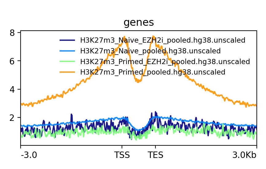
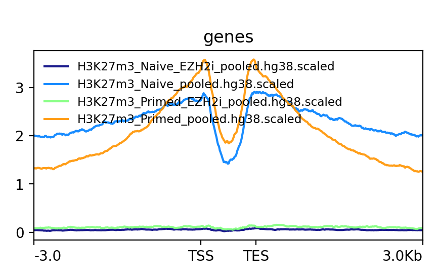
This is an example of how the pooled replicates look on average. As you can see, when not scaled, Primed looks like it is much more enriched at bivalent genes than Naïve. This difference becomes much smaller when scaled.
Q: How do the scaled Naïve vs Primed differ when you move away from the gene body?
You can check this by playing with the parameters --downstream and --upstream when running computeMatrix.
Example command
computeMatrix scale-regions --downstream 5000 --upstream 5000 -S ./bw/H3K27*pooled.hg38.scaled.bw -R Bivalent_Court2017.hg38.bed -o bivalent_mat_scaled.npz --outFileNameMatrix bivalent_values_scaled.tab -p 4
Q: How do the scaled vs unscaled plots differ? What do you think that means?
Explanation
What is making all the difference is the real H3K27m3 background across the genome. You see in the scaled plots that Naïve is higher across. So what happens is that the “peaks” in naïve look smaller with such background, and if there is no absolute scaling that makes it possible to compare Naïve vs Primed, Naïve looks flat, as you saw in the unscaled plot. An additional control to make sure this is not technical background is the EZH2i treatment, which removes pretty much all H3K27m3 genome-wide.
Q: Is this a general effect, or is it dominated by a few loci?
Hint: You can look at this using deepTools plotHeatmap function. It will take as input the matrix you calculated with computeMatrix and generate a heatmap.
Genome-wide bin distribution
Another way of looking at the general effect of the scaling genome-wide is using deepTools multiBigwigSummary tool to generate bin average profiles genome-wide and look at their
distribution.
multiBigwigSummary bins -b ./bw/H3K27*pooled.hg38.scaled.bw ./bw/H3K27*pooled.hg38.unscaled.bw -o 10kb_bins.npz --outRawCounts 10kb_bins.tab -bs 10000 -p 4
This will generate a 10kb_bins.tab tab-delimited file that contains mean coverage per 10kb bin across the genome for the different bigWig files. You can import this table into R and look at the bin distribution using some simple ggplot commands.
Note
Since you already have run RStudio in other tutorials, you can use any approach you have used before for running R. Just note that you need to have access to this 10kb_bins.tab you just created. You can also do it locally in your computer, if you have a RStudio version installed, and you will only need ggplot2 and GenomicRanges + rtracklayer.
First, import the data into a data frame:
# Note it is important the :code:`comment.char` parameter, as deepTools inserts a :code:`#`,
# which is the default comment in R, so it will not read the header properly otherwise
df <- read.table("./10kb_bins.tab", header=T, sep= "\t", comment.char = "")

# You can check that this has reasonable names
colnames(df)
We can make this a little more readable:
colnames(df) <- c(
  c("seqnames", "start", "end"),
  gsub("_rep1.hg38|.bw", "", colnames(df)[4:ncol(df)])
)

colnames(df)
So we can for instance check the differences scaled vs unscaled in a scatterplot:
library(ggplot2)

ggplot(df, aes(x=H3K27m3_Naive.unscaled, y=H3K27m3_Primed.unscaled)) +
  geom_point(alpha = 0.4) +
  coord_cartesian(xlim=c(0,30), ylim=c(0,30))


ggplot(df, aes(x=H3K27m3_Naive.scaled, y=H3K27m3_Primed.scaled)) +
  geom_point(alpha = 0.4) +
  coord_cartesian(xlim=c(0,30), ylim=c(0,30))
Resulting figures
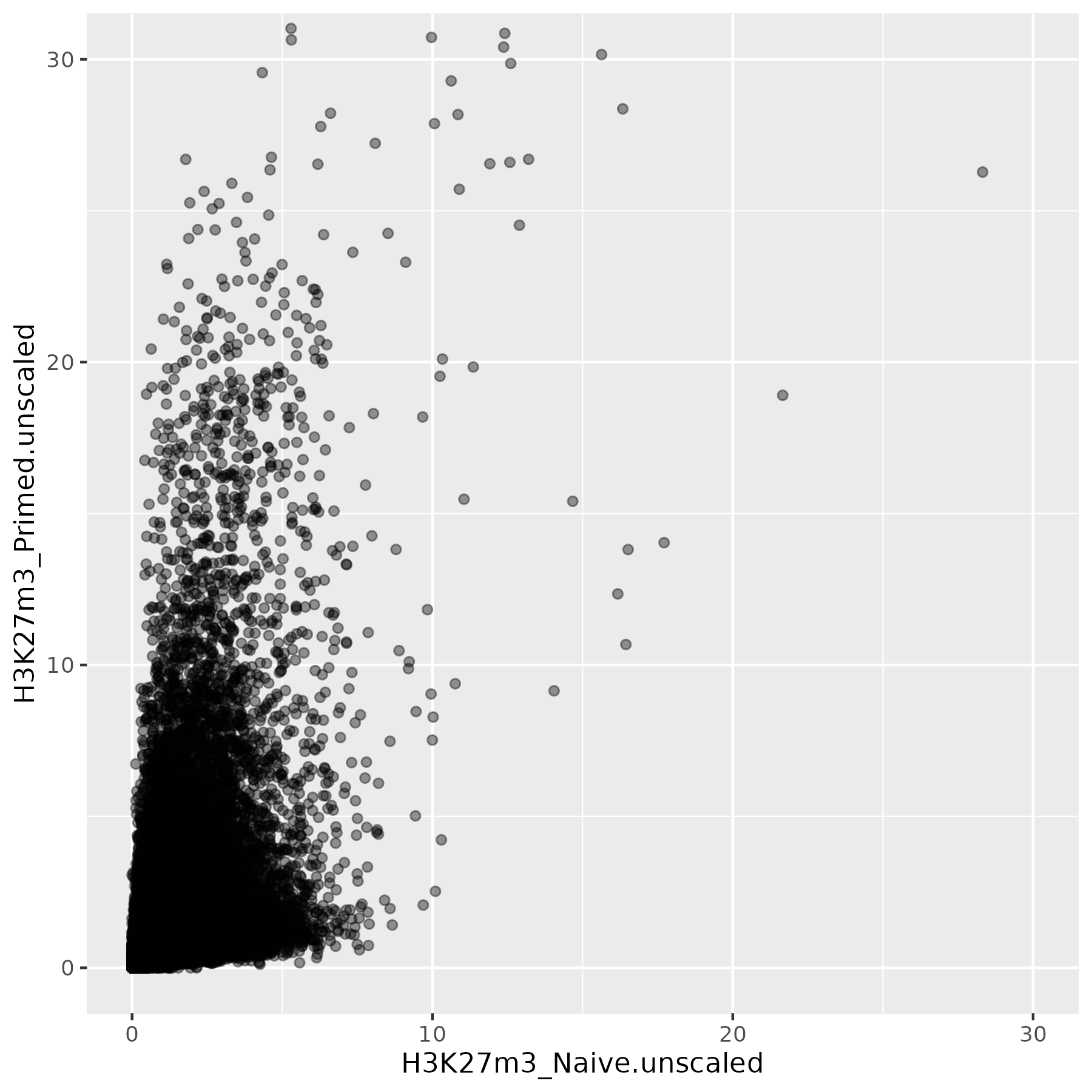
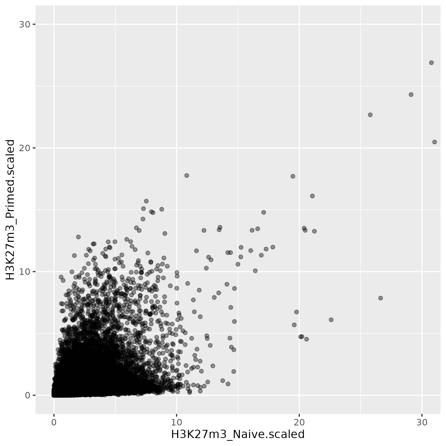
This is not the most striking of figures, but what you can already see is that there are a bunch of 10kb bins that look super high in Primed compared to Naïve when looking at unscaled data, and that large difference drops a lot when the datapoints are scaled. Still, there is heterogeneity, and it requires a deeper analysis to understand what’s happening in detail.
We can make a GRanges object with these values and perform
some operations, like check which bins overlap with some annotation, and things like this.
library(GenomicRanges)
library(rtracklayer)

gr <- makeGRangesFromDataFrame(df, keep.extra.columns = T)
bivalent <- import("./Bivalent_Court2017.hg38.bed")

biv_bins <- subsetByOverlaps(gr, bivalent)

# You can use this data frame to plot only the bivalent-overlapping bins
biv_df <- data.frame(biv_bins)
So we could be interested in plotting only bins that overlap with bivalent genes, and many other things. In this case, bins are somewhat large, so they will not represent exactly the annotations that we plotted in the previous step.
The same way we generated these figures, there are a lot of things that can be done, and many questions can be addressed, for instance:
Do you think that the bin size affects this type of analysis in deeper ways? How different would these figures look if the bin size was 5kb? Which size would you think is a good compromise without getting a difficult to handle number of data points?
How is the distribution of values per chromosome? Hint: look again at the tracks in the primary analysis part!
Appendix: Interferences between conda and the module system
As a side note, there can be sometimes interference between conda environments and the Uppmax module system, so if you don’t follow the tutorial in order, which could happen (e.g you might want to go see the bigWig files while you wait for the minute primary analysis to run), you might run into some issues.
Problem: I tried to resume a minute run and now it does not run and I get some kind of python exception, most
likely ModuleNotFoundError … No module named XYZ.
Solution: In my experience this has happened when I loaded module load deepTools and tried
to use the conda environment after. A quick check on which python yields a path
that is not in the conda environment directory, but a system-wide installation of
python. module list will show you a list of modules
that are loaded and very likely there will be deepTools in it.
My recommendation is to unload everything using module unload
(or log-out and log-in to your node again might also work) and restart, module load bioinfo-tools,
module load conda, conda activate and then try to run minute again.